
GGR 274 Review (Weeks 7-11)#
Week 7: Probability and Statistical Distributions
Week 8: Statistical Inference
Week 9: Correlation & Regression
Week 10: Spatial Data & Mapping
Week 11: Spatial Analysis
Coding Concepts#
import pandas as pd

df = pd.read_csv("ggr274_survey.csv")

df.head()
.groupby("column"): Group data frame based on one or more columns (for example, creating groups of survey respondents that prefer each season).groupby("column").size(): Count number of observations in each group
df.groupby("favourite_season")
df.groupby("favourite_season").size()
.groupby(["column1", "column2"]).size().unstack(): Get these results in a table
counts = df.groupby(["favourite_season", "commute_mode"]).size().unstack()

counts
.sum(): sum column or row.sum(axis = 0): Sum each column.sum(axis = 1): Sum each row
counts.sum(axis = 0)
counts.sum(axis = 1)
.div(): divide column or row by total.div(.sum(axis = 0), axis = 1): Divide each value by the sum of the column.div(.sum(axis = 1), axis = 0): Divide each value by the sum of the rows
counts.div(counts.sum(axis = 0), axis = 1)
counts.div(counts.sum(axis = 1), axis = 0)
.loc[]:df.loc[2]pulls the third row from a data frame
df.loc[2]
df.loc[boolean_list]ordf.loc[df["condition"] == True]pulls rows where boolean condition isTrue
winter_boolean = df["favourite_season"] == "Winter"

df.loc[winter_boolean]
df.loc[df["favourite_season"] == "Winter"]
def(): define a function, ending withreturn
import random

def roll_six_sided_die():
    ''' Simulate the roll of a six-sided die by returning a number
        between 1 and 6
    '''
    roll = random.randint(1, 6)
    return roll
roll_six_sided_die()
.merge()left=: first data frameright=: second data frameleft_on=: merge column from first data frameright_on=: merge column from second data framehow=: keeping all rows from first data frame ("left"), from the second data frame ("right"), from either data frame ("outer"), or from both data frames ("inner")
Week 7: Probability and Statistical Distributions#
How to calculate a frequency table with
.value_counts().sort_index()How to calculate probabilities (likelihoods that each outcome will occur) from a frequency table
How to generate a random sample and simulate a distribution with
.sample()How to plot a distribution using
.plot.bar()and.plot.hist(), and when you would use eachCalculating population mean and population standard deviation using
.mean()andstatistics.pstdev()
Week 8: Statistical Inference#
Calculating sample mean and sample standard deviation using
.mean()and.std()Calculating standard error, margin of error, and confidence interval
\(SE = s/\sqrt{n}\)
\(MOE = z * SE\)
\(CI = \bar{x} \pm MOE\)
What factors can increase these measures (indicating less certainty) or decrease these measures (indicating greater certainty)?
Constructing a hypothesis test
Null Hypothesis (\(H_0\))
Alternative Hypothesis (\(H_a\))
Calculating and interpreting statistics from one-sample and two-sample t-tests
One-sample t-test:
stats.ttest_1samp(sample, popmean = population_mean, alternative="___")Two-sample t-test:
stats.ttest_ind(sample1, sample2, equal_var=False, alternative="___")
Week 9: Correlation & Regression#
Calculating and interpreting correlation with
statistics.correlation()Running and interpreting the output of a linear regression produced via
ols().fit()Interpretation of regression coefficients (intercept and slope)
Interpretation of t-statistics and p-values associated with regression coefficients
Interpretation of \(R^2\) value
Week 10: Spatial Data & Mapping#
Types of spatial data (raster, vector, point, line, polygon)
Structure of
geopandasGeoDataFramesHow to create side-by-side thematic maps using
plt.subplots()and.plot()
Types and uses of different map colour palettes
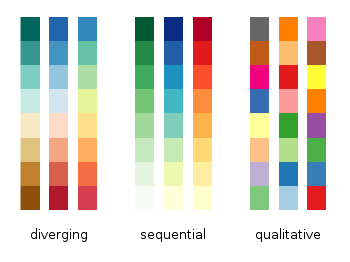
Types and uses of different map classification schemes
Equal Intervals
Quantile
Natural Breaks (Fisher/Jenks)
Week 11: Spatial Analysis#
Purpose of Coordinate Reference Systems (CRS) and reasons to alter the CRS
Accurate measurement
Alignment with other datasets
Spatial measurement (
.area,.length, and.distance)Plotting maps with multiple layers
Spatial processing:
Clipping (
.clip()): getting rid of spatial components that do not overlapBuffers (
.buffer()): generating an area within a certain distance of a geometrySpatial Joins
.sjoin()and.drop_duplicates()): joining together two GeoDataFrames with geometries that overlap in space.merge()to join a GeoDataFrame with a non-spatial DataFrame based on any column(s) they have in common
Where to go from here?#
This course provides you with the fundamental tools for conducting data analysis to ask social science questions.
There are many additional tools we have not explored!
Advanced topics in Python
More complex data wrangling such as
.apply(),map(), andfilter()More complex functions from various packages
Advanced statistical methods
More regression models (other than linear regression)
How to prove causality (i.e. X causes Y), rather than just measuring associations
Machine learning (identifying categories, optimizing predictions)
Advanced spatial methods
Cluster and hotspot analysis
Spatial statistics (such as spatial regression)