Class 7: Different ways to select data

Class 7: Different ways to select data#

Last class:

Introduced .groupby() and .loc[]
Started talking about visualizing data

This class:

How to identify rows by “index”
Subsetting rows (and columns) using .loc[]
Reviewing .groupby()
Creating simple plots

We will use our class survey data to keep things simple

import pandas as pd

class_data = pd.read_csv("ggr274_survey.csv")
class_data.head()

	id	year	specialist_major	drink_type	cups_per_week	favourite_season	pets_num	pets_type	commute_mode	commute_time	intersection	city
0	1	3.0	Economics	Tea	5	Fall	0	NaN	Walking/Rolling	30	King and Spadina	Toronto
1	2	3.0	Biodiversity and Conservation Biology	Tea	4	Summer	0	NaN	Walking/Rolling	15	Bay Street and Wellesley Street	Toronto
2	3	2.0	Finance and Economics Specialist	Coffee	2	Summer	3	Dog;	Walking/Rolling	10	Spadina Avenue & Harbour Street	Toronto
3	4	2.0	B.M. Violin performance	Coffee	12	Summer	0	NaN	Subway	60	Major Mackenzie & Hwy 7	Toronto
4	5	2.0	Sociology	Tea	3	Fall	0	NaN	Walking/Rolling	15	Bay Street & Bloor Street	Toronto

Index#

We use the term “index” in a particular way with Pandas DataFrames. It is used to identify rows in the table.

By default the index is a range starting at 0. You can see it as the unlabeled left-most column above.

It is also an attribute of the DataFrame

class_data.index

RangeIndex(start=0, stop=62, step=1)

You can change the index by setting it to a different column. Notice that how the view of the data frame changes.

class_data_id = class_data.set_index("id")

class_data_id.head()

	year	specialist_major	drink_type	cups_per_week	favourite_season	pets_num	pets_type	commute_mode	commute_time	intersection	city
id
1	3.0	Economics	Tea	5	Fall	0	NaN	Walking/Rolling	30	King and Spadina	Toronto
2	3.0	Biodiversity and Conservation Biology	Tea	4	Summer	0	NaN	Walking/Rolling	15	Bay Street and Wellesley Street	Toronto
3	2.0	Finance and Economics Specialist	Coffee	2	Summer	3	Dog;	Walking/Rolling	10	Spadina Avenue & Harbour Street	Toronto
4	2.0	B.M. Violin performance	Coffee	12	Summer	0	NaN	Subway	60	Major Mackenzie & Hwy 7	Toronto
5	2.0	Sociology	Tea	3	Fall	0	NaN	Walking/Rolling	15	Bay Street & Bloor Street	Toronto

# Now the index is defined as a list

class_data_id.index

Index([ 1,  2,  3,  4,  5,  6,  7,  8,  9, 10, 11, 12, 13, 14, 15, 16, 17, 18,
       19, 20, 21, 22, 23, 24, 25, 26, 27, 28, 29, 30, 31, 32, 33, 34, 35, 36,
       37, 38, 39, 40, 41, 42, 43, 44, 45, 46, 47, 48, 49, 50, 51, 52, 53, 54,
       55, 56, 57, 58, 59, 60, 61, 62],
      dtype='int64', name='id')

We could continue working with our new index, but since we are not often going to redefine the index in this class, we will keep it simple and go back to our default state. The DataFrame class_data hasn’t changed.

The reason to talk about a DataFrame’s index is because the way we select rows is based on the index. Before we jump into that, let’s quickly review how we select columns from the DataFrame

class_data.head()

	id	year	specialist_major	drink_type	cups_per_week	favourite_season	pets_num	pets_type	commute_mode	commute_time	intersection	city
0	1	3.0	Economics	Tea	5	Fall	0	NaN	Walking/Rolling	30	King and Spadina	Toronto
1	2	3.0	Biodiversity and Conservation Biology	Tea	4	Summer	0	NaN	Walking/Rolling	15	Bay Street and Wellesley Street	Toronto
2	3	2.0	Finance and Economics Specialist	Coffee	2	Summer	3	Dog;	Walking/Rolling	10	Spadina Avenue & Harbour Street	Toronto
3	4	2.0	B.M. Violin performance	Coffee	12	Summer	0	NaN	Subway	60	Major Mackenzie & Hwy 7	Toronto
4	5	2.0	Sociology	Tea	3	Fall	0	NaN	Walking/Rolling	15	Bay Street & Bloor Street	Toronto

# recall how we select columns from a DataFrame

# select one column
class_spec = class_data["specialist_major"]
print(class_spec)

# what data type do we get as a result?
print(type(class_spec))

                              Economics 
   Biodiversity and Conservation Biology
       Finance and Economics Specialist 
                 B.M. Violin performance
                               Sociology
                      ...                  
                 Finance and Economics 
                      Civil Engineering
                             Management
                                 Rotman
                              Sociology
Name: specialist_major, Length: 62, dtype: object
<class 'pandas.core.series.Series'>

# also notice that a Series has an index

class_spec.index

RangeIndex(start=0, stop=62, step=1)

# select multiple columns
class_data[["specialist_major", "commute_mode"]]

	specialist_major	commute_mode
0	Economics	Walking/Rolling
1	Biodiversity and Conservation Biology	Walking/Rolling
2	Finance and Economics Specialist	Walking/Rolling
3	B.M. Violin performance	Subway
4	Sociology	Walking/Rolling
...	...	...
57	Finance and Economics	Walking/Rolling
58	Civil Engineering	Bicycle/Scooter
59	Management	Walking/Rolling
60	Rotman	Walking/Rolling
61	Sociology	Walking/Rolling

62 rows × 2 columns

Selecting rows#

The .loc[] accessor allows us to do a similar selection for rows. Here is how we select a single row by its index.

What data type do we get?

class_row = class_data.loc[2]

print(class_row)

print(type(class_row))

id                                                  3
year                                              2.0
specialist_major    Finance and Economics Specialist 
drink_type                                     Coffee
cups_per_week                                       2
favourite_season                               Summer
pets_num                                            3
pets_type                                        Dog;
commute_mode                          Walking/Rolling
commute_time                                       10
intersection          Spadina Avenue & Harbour Street
city                                         Toronto 
Name: 2, dtype: object
<class 'pandas.core.series.Series'>

Wait, that’s a Series? It doesn’t really look like the Series we saw above. Is the first column really an index?

When we select a single row, we get a Series that is the values in the row. The Index for this series is the column headings.

class_data.loc[2].index

Index(['id', 'year', 'specialist_major', 'drink_type', 'cups_per_week',
       'favourite_season', 'pets_num', 'pets_type', 'commute_mode',
       'commute_time', 'intersection', 'city'],
      dtype='object')

Selecting multiple rows#

There are several ways to do this. Similar to selecting columns, the result of selecting multiple rows is a DataFrame.

We can use the same method as we did for selecting multiple columns by just passing in a list.
If the index is a Range, then we can also use list slicing to select rows.

# select multiple rows

class_data.loc[[2, 4]]

	id	year	specialist_major	drink_type	cups_per_week	favourite_season	pets_num	pets_type	commute_mode	commute_time	intersection	city
2	3	2.0	Finance and Economics Specialist	Coffee	2	Summer	3	Dog;	Walking/Rolling	10	Spadina Avenue & Harbour Street	Toronto
4	5	2.0	Sociology	Tea	3	Fall	0	NaN	Walking/Rolling	15	Bay Street & Bloor Street	Toronto

# because the index in this case is a range, we can also use list slicing to get a range

class_data.loc[2:4]

	id	year	specialist_major	drink_type	cups_per_week	favourite_season	pets_num	pets_type	commute_mode	commute_time	intersection	city
2	3	2.0	Finance and Economics Specialist	Coffee	2	Summer	3	Dog;	Walking/Rolling	10	Spadina Avenue & Harbour Street	Toronto
3	4	2.0	B.M. Violin performance	Coffee	12	Summer	0	NaN	Subway	60	Major Mackenzie & Hwy 7	Toronto
4	5	2.0	Sociology	Tea	3	Fall	0	NaN	Walking/Rolling	15	Bay Street & Bloor Street	Toronto

Using Boolean expressions to select rows#

Once again this works the same as how we used these series on columns.

# use a boolean expression to select rows

# construct a boolean series that is true for the rows where "drink_type" is "Tea"
drink_type = class_data["drink_type"] == "Tea"

# Use the new series to subset the DataFrame
class_data.loc[drink_type]

	id	year	specialist_major	drink_type	cups_per_week	favourite_season	pets_num	pets_type	commute_mode	commute_time	intersection	city
0	1	3.0	Economics	Tea	5	Fall	0	NaN	Walking/Rolling	30	King and Spadina	Toronto
1	2	3.0	Biodiversity and Conservation Biology	Tea	4	Summer	0	NaN	Walking/Rolling	15	Bay Street and Wellesley Street	Toronto
4	5	2.0	Sociology	Tea	3	Fall	0	NaN	Walking/Rolling	15	Bay Street & Bloor Street	Toronto
6	7	4.0	Economics	Tea	6	Summer	1	Cat;	Walking/Rolling	30	King W and Spadina	Toronto
8	9	2.0	Economics	Tea	0	Summer	0	NaN	Walking/Rolling	25	Yonge Street & Bloor Street	Toronto
9	10	2.0	Linguistics	Tea	1	Fall	0	NaN	Bicycle/Scooter	10	Davenport Road & Avenue Road	Toronto
11	12	3.0	Human Geography	Tea	4	Fall	1	Cat;	Walking/Rolling	5	Bloor Street & St George Street	Toronto
12	13	3.0	Specialist in Finance and Econ	Tea	0	Fall	0	NaN	Walking/Rolling	25	Yonge and Bloor	Toronto
13	14	3.0	Economics	Tea	0	Spring	0	NaN	Bicycle/Scooter	20	Bloor and Sherborne	Toronto
17	18	2.0	Political Science	Tea	0	Fall	1	Dog;	Subway	50	Keele & Sheppard Avenue West	Toronto
19	20	NaN	Rotman Commerce Specialist Finance and Economics	Tea	4	Summer	0	NaN	Walking/Rolling	10	Bloor and Avenue Road	Toronto
20	21	2.0	Urban studies	Tea	12	Spring	2	Cat;Dog;	Subway	60	Keele Street & Sheppard Ave West	Toronto
27	28	4.0	Philosophy	Tea	2	Spring	1	Cat;	Walking/Rolling	15	Avenue Street and Bloor Street	Toronto
28	29	3.0	Environmental Geography	Tea	3	Summer	1	Cat;	Walking/Rolling	20	Bay Street & Charles Street	Toronto
29	30	1.0	Psychology and Linguistics	Tea	7	Fall	1	Dog;	Subway	90	Bayview Ave & Major Mackenzie Ave	Richmond Hill
30	31	4.0	Accounting	Tea	3	Fall	0	NaN	Walking/Rolling	10	College and Spadina	Toronto
31	32	4.0	Economics	Tea	3	Spring	0	NaN	Walking/Rolling	20	Bay Street & College Street	Toronto
33	34	3.0	Rotman Commerce Finance and Economics Specialist	Tea	2	Summer	1	Dog;	Subway	60	Bay & Bloor	Toronto
36	37	4.0	Archaeology	Tea	10	Spring	0	NaN	Subway	60	Dixie and Queensway	Mississauga
38	39	2.0	Political Science	Tea	3	Spring	0	NaN	Walking/Rolling	12	Avenue Road and Bloor	Toronto
41	42	3.0	Cognitive Science	Tea	1	Spring	0	NaN	Subway	45	Yonge Street & Empress Avenue	Toronto
44	45	4.0	Civil Engineering	Tea	3	Summer	0	NaN	Subway	30	Yonge Street & Eglinton Ave	Toronto
49	50	4.0	Geography	Tea	1	Spring	0	NaN	Walking/Rolling	20	Bloor	Toronto
58	59	4.0	Civil Engineering	Tea	0	Summer	0	NaN	Bicycle/Scooter	15	Bay Street & Bloor Street	Toronto
59	60	2.0	Management	Tea	5	Fall	1	Cat;	Walking/Rolling	12	Bay Street & Bloor Street	Toronto
61	62	1.0	Sociology	Tea	3	Spring	0	NaN	Walking/Rolling	13	College Street & Spadina Avenue	Toronto

Back to .groupby()#

What kinds of questions can we answer using .groupby()

Grouby statements follow a pattern:

df.groupby("category")["column of interest"].aggregator()

Where df is the dataframe, "category" is the field by which we want to divide up the data, "column of interest" is the column we want to do the math on, and aggregator is the function we want to apply. Let’s look at a few examples:

Question 1: How many students prefer each season?

# There are two ways to do this that we've seen
# The first doesn't use .groupby, it uses .value_counts()

class_data["favourite_season"].value_counts()

favourite_season
Summer    24
Fall      21
Spring    12
Winter     5
Name: count, dtype: int64

# Using groupby

# We use size instead of count because count will give us a table with a count for each column (try it out)

class_data.groupby("favourite_season").size()

favourite_season
Fall      21
Spring    12
Summer    24
Winter     5
dtype: int64

Question 2: Does commute time depend on mode of travel?

Let’s think about this step by step:

group by commute mode
select the commute time column
decide how to aggregate - In this case we want to find the mean commute time for a given mode of travel

class_data.groupby("commute_mode")["commute_time"].mean()

commute_mode
Bicycle/Scooter    15.000000
Car                45.000000
Subway             53.125000
Walking/Rolling    17.595238
Name: commute_time, dtype: float64

Question 3: For each season, how many people prefer each drink type?

This question is a little different because we want to compare two categories, so we will select both categories. The first method gives us a kind of nested table which is a little hard to work with. In the second approach we use “unstack” to get a DataFrame we can work with. Before we get to the second example, we will clean up the data a bit too.

class_data.groupby(["favourite_season", "drink_type"]).size()

favourite_season  drink_type   
Fall              Coffee            9
                  Hot Chocolate     1
                  Hot chocolate     1
                  Juice             1
                  Tea               9
Spring            Coffee            3
                  Tea               9
Summer            Coffee           15
                  Hot Chocolate     1
                  Tea               8
Winter            Coffee            3
                  Matcha            1
                  hot chocolate     1
dtype: int64

# We really should clean up the drink_type column, so that we don't have multiple versions of "hot chocolate"

# Reassign the values in the "drink_type" column
# strip the white space from around the string
# set each one to lower case

class_data["drink_type"] = (
    class_data["drink_type"]
        .str.strip()
        .str.lower()
)

# If we want this as a table, then we need to unstack it

class_data.groupby(["favourite_season", "drink_type"]).size().unstack()

drink_type	coffee	hot chocolate	juice	matcha	tea
favourite_season
Fall	9.0	2.0	1.0	NaN	9.0
Spring	3.0	NaN	NaN	NaN	9.0
Summer	15.0	1.0	NaN	NaN	8.0
Winter	3.0	1.0	NaN	1.0	NaN

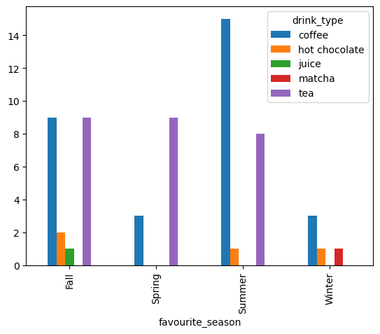
# Assign the result to a variable so we can plot it

counts = (
    class_data.groupby(["favourite_season", "drink_type"])
      .size()
      .unstack()
)

counts.plot(kind="bar")

<Axes: xlabel='favourite_season'>

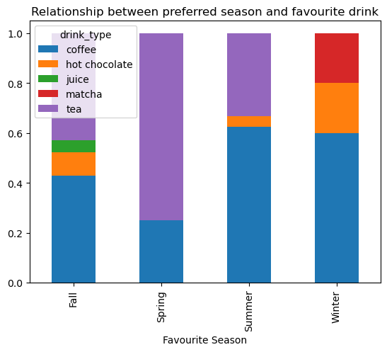
../../../_images/46e9e791ca73acf6179c4ce8ab139d2dbd3b206d1831be810ee6f08fa3227fef.png

But we probably want proportions rather than counts. Let’s take this step by step.

For each season we would like to know what proportion each drink makes up for the drinks for that season

\[ \text{proportion} = \frac{\text{count of a single drink for that season}} {\text{total number of drinks for that season}} \]

Step 1: Given counts, we need to sum up the number of drinks for each season.

axis=1 means go across the columns. In other words we want the sum of the values in a row.

counts.sum(axis=1)

favourite_season
Fall      21.0
Spring    12.0
Summer    24.0
Winter     5.0
dtype: float64

Step 2: Now we can divide by each cell by its row total

counts.div(counts.sum(axis=1), axis=0)

Using the .div() aggregator method, divide every cell by the total for that’s cell’s row. The total is given by counts.sum(axis=1), and axis=0 tells the aggregator to go across the rows. So each season’s row is divided by its own total.

proportions = counts.div(counts.sum(axis=1), axis=0)
print(proportions)

drink_type          coffee  hot chocolate     juice  matcha       tea
favourite_season                                                     
Fall              0.428571       0.095238  0.047619     NaN  0.428571
Spring            0.250000            NaN       NaN     NaN  0.750000
Summer            0.625000       0.041667       NaN     NaN  0.333333
Winter            0.600000       0.200000       NaN     0.2       NaN

# Let's plot this one

proportions.plot(kind="bar", 
                 stacked=True, 
                 title="Relationship between preferred season and favourite drink" ,
                 xlabel="Favourite Season")

<Axes: title={'center': 'Relationship between preferred season and favourite drink'}, xlabel='Favourite Season'>

../../../_images/d8c0e541abb45dd6def29f0205cc66018887c957c78639a82109eb5381260f4c.png