
Lecture 8: Statistical Inference#
Review: Statistical Distributions#
Last time, we discussed statistical distributions: mathematical and graphical representations of the likelihood that different outcomes occur. Some of these distributions can consistently describe the likelihood of real-world phenomena, such as:
Binomial: Likelihood of a binary event happening a certain number of times in a certain number of attempts
Poisson: Likelihood of an event occurring a certain number of times during a fixed period
Normal: Likelihood of getting a particular value from a continuous distribution
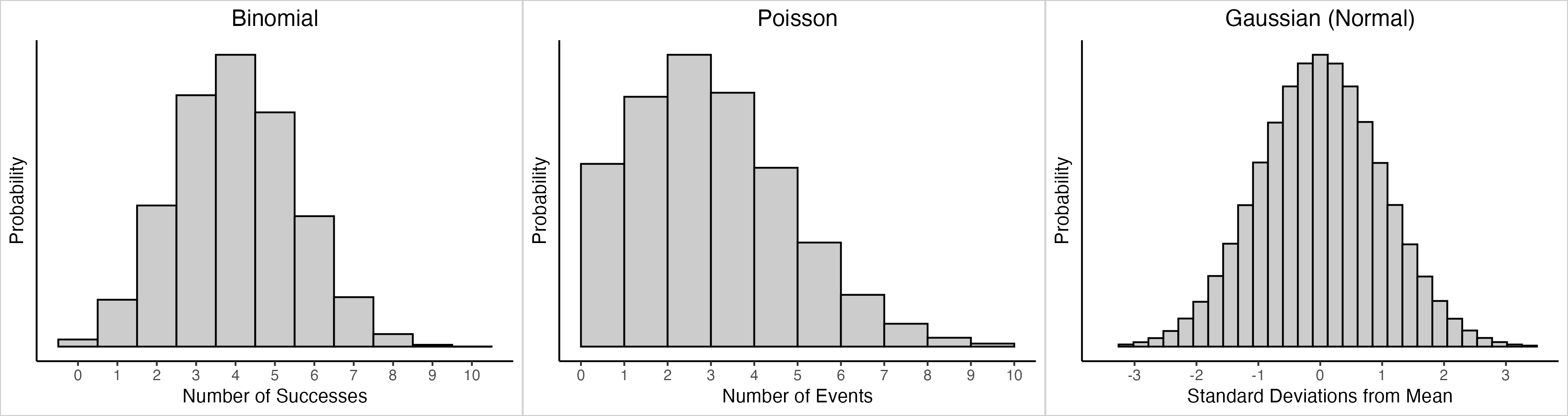
Why are these abstract statistical distributions useful for the social sciences?
One big reason is that these distributions allow us to infer (figure out from existing evidence) information about an entire population from a limited sample.
This technique is also known as “statistical inference”!
For today’s example, let’s look at the data from the General Social Survey, which contains 12,336 observations.
import pandas as pd

gss = pd.read_csv("gss_2022.csv")

gss.shape
Let’s focus on the column SLEEPDUR, which tells us how many minutes respondents sleep each night:
gss["SLEEPDUR"]
To make this easier to interpret, let’s create a new object called sleep_hours that translates this into hours
sleep_hours = gss["SLEEPDUR"]/60

sleep_hours
Let’s calculate the mean and standard deviation of this variable, using the formulas from last week:
sleep_hours_mean = sum(sleep_hours)/len(sleep_hours)

sleep_hours_sd = (sum((sleep_hours - sleep_hours_mean)**2)/(len(sleep_hours)))**0.5

print(round(sleep_hours_mean, 2))

print(round(sleep_hours_sd, 2))
Let’s plot the distribution of this variable. We’ll also add a vertical red line marking the mean, and use plt.figtext to add labels indicating the mean and standard deviation.
import seaborn as sns
import matplotlib.pyplot as plt

sns.histplot(sleep_hours, bins = range(0, 25)).axvline(sleep_hours_mean, color = "red")

plt.figtext(0.5, 0.8, f"Population Mean = {round(sleep_hours_mean, 2)}", color = "red")
plt.figtext(0.5, 0.75, f"Population SD = {round(sleep_hours_sd, 2)}", color = "red")
Sampling#
Let’s say that we didn’t have enough resources to go out and survey all 12,000+ survey respondents. What if we were only able to get answers from 100 of them?
Last time, we discussed how to use .sample() to select random entries from a list. This time, we’ll use the same function to select 100 random responses from our survey (<1%).
replace = False is used so that we don’t draw the same survey response multiple times!
sleep_hours_sample = sleep_hours.sample(100, replace = False)

sleep_hours_sample
While the mean of a population is symbolized by \(\mu\), the mean of a sample is represented by \(\bar{x}\). The formulas for these are almost exactly the same, but there are important conceptual differences.
The capital \(N\) indicates the size of the total population, whereas the lowercase \(n\) indicates the size of the sample.
The standard deviation of a population (\(\sigma\)) is also distinct from the population of a sample (\(s\)):
The sample standard deviation divides by \(n - 1\) instead of \(N\). There are important mathematical reasons for this, but we won’t get into that here!
As with the full population, we can manually calculate the mean and standard deviation for our sample.
This time, however, because it’s a sample, we will use \(n - 1\) for standard deviation!
sleep_hours_sample_mean = sum(sleep_hours_sample)/len(sleep_hours_sample)

sleep_hours_sample_sd = (sum((sleep_hours_sample - sleep_hours_sample_mean)**2)/(len(sleep_hours_sample) - 1))**0.5

print(sleep_hours_sample_mean)
print(sleep_hours_sample_sd)
Instead of calculating this manually, the built-in pandas function for standard deviation .std() automatically calculates the sample standard deviation (including the \(n - 1\)).
We can use .mean() and .std() to calculate the mean and standard deviation of our last sample!
print(sleep_hours_sample.mean())

print(sleep_hours_sample.std())
With those tools in hand, let’s look at how the distribution, mean, and standard deviation change each time we resample our data.
sleep_hours_sample = sleep_hours.sample(100, replace = False)

sleep_hours_sample_mean = sleep_hours_sample.mean()
sleep_hours_sample_sd = sleep_hours_sample.std()

sns.histplot(sleep_hours, bins = range(0, 25)).axvline(sleep_hours_sample_mean, color = "red")

plt.figtext(0.5, 0.8, f"Population Mean = {round(sleep_hours_mean, 2)}", color = "red")
plt.figtext(0.5, 0.75, f"Sample Mean = {round(sleep_hours_sample_mean, 2)}", color = "red")
plt.figtext(0.5, 0.65, f"Population SD = {round(sleep_hours_sd, 2)}", color = "red")
plt.figtext(0.5, 0.6, f"Sample SD = {round(sleep_hours_sample_sd, 2)}", color = "red")
Simulating Statistics#
Each time we take sample from our survey data, it has a different distribution and a different mean. And each of these are a little bit different from the “true” mean of the surveyed population!
This is a huge problem. If taking different samples from a population can produce different results, how can we possibly use survey data to get an accurate picture?
Some samples could be pretty representative of the overall population, but others might be super different!
One way to fix this is to increase the size of our sample. As the size of the random sample increases, each sample will increasingly resemble the overall population.
sleep_hours_sample = sleep_hours.sample(6000, replace = False)

sleep_hours_sample_mean = sleep_hours_sample.mean()
sleep_hours_sample_sd = sleep_hours_sample.std()

sns.histplot(sleep_hours, bins = range(0, 25)).axvline(sleep_hours_sample_mean, color = "red")

plt.figtext(0.5, 0.8, f"Population Mean = {round(sleep_hours_mean, 2)}", color = "red")
plt.figtext(0.5, 0.75, f"Sample Mean = {round(sleep_hours_sample_mean, 2)}", color = "red")
plt.figtext(0.5, 0.65, f"Population SD = {round(sleep_hours_sd, 2)}", color = "red")
plt.figtext(0.5, 0.6, f"Sample SD = {round(sleep_hours_sample_sd, 2)}", color = "red")
In practice, it often isn’t practical to simply increase the sample size. Surveys are expensive!
Besides, there is another way that we can approximate the “true” mean (or at least quantify our uncertainty about a particular sample):
Simulation, also known in this context as Bootstrapping.
We did some simulation last week, when we did 10 coin flips (or 2 dice rolls) a bunch of times in a row.
This time we’re going to do something very similar. Except that instead of flipping a coin, we’re going to pull a bunch of random samples of 100 people from our survey data!
For each sample, we will calculate the mean value, and add it to our list of sample means
sample_means = []

for i in range(10000):
    sleep_hours_sample = sleep_hours.sample(n = 100, replace = False, random_state = i)
    sample_means.append(sleep_hours_sample.mean())

sample_means = pd.Series(sample_means)

sample_means
The sample_means list contains the means from 10,000 random samples of 120 observations. What happens if we plot the distribution of these sample means?
sns.histplot(sample_means).axvline(sample_means.mean(), color = "red")
This is starting to look like a normal distribution!
Just like with rolling a bunch of dice: the more dice we add, the closer the total comes to a normal distribution.
In this case, the more samples we take of the data, the more closely the means of those samples conform to a normal distribution.
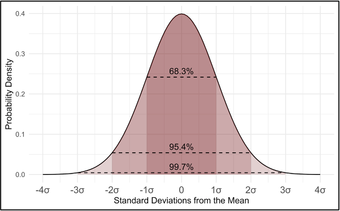
Because sample means are normally distributed, we can use the fundamental characteristics of normal distributions to figure out how likely we are to find the “true” population mean!
mean_of_sample_means = sample_means.mean()
sd_of_sample_means = sample_means.std()

print(round(mean_of_sample_means, 2))
print(round(sd_of_sample_means, 2))
print(f"There is a 68.3% likelihood that the true population mean is located between {round(mean_of_sample_means - sd_of_sample_means, 2)} and {round(mean_of_sample_means + sd_of_sample_means, 2)}")
print(f"There is a 95.4% likelihood that the true population mean is located between {round(mean_of_sample_means - 2*sd_of_sample_means, 2)} and {round(mean_of_sample_means + 2*sd_of_sample_means, 2)}")
print(f"There is a 99.7% likelihood that the true population mean is located between {round(mean_of_sample_means - 3*sd_of_sample_means, 2)} and {round(mean_of_sample_means + 3*sd_of_sample_means, 2)}")
Oftentimes, we will use specific multiples of standard deviations to get specific levels of likelihood:
Likelihood |
Standard Deviations from Mean |
|---|---|
80% |
\(\mu\ \pm\) 1.28 \(\sigma\) |
90% |
\(\mu\ \pm\) 1.645 \(\sigma\) |
95% |
\(\mu\ \pm\) 1.96 \(\sigma\) |
99% |
\(\mu\ \pm\) 2.58 \(\sigma\) |
mean_of_sample_means = sample_means.mean()
sd_of_sample_means = sample_means.std()

print(f"There is a 80% likelihood that the true population mean is located between {round(mean_of_sample_means - 1.28*sd_of_sample_means, 2)} and {round(mean_of_sample_means + 1.28*sd_of_sample_means, 2)}")
print(f"There is a 90% likelihood that the true population mean is located between {round(mean_of_sample_means - 1.645*sd_of_sample_means, 2)} and {round(mean_of_sample_means + 1.645*sd_of_sample_means, 2)}")
print(f"There is a 95% likelihood that the true population mean is located between {round(mean_of_sample_means - 1.96*sd_of_sample_means, 2)} and {round(mean_of_sample_means + 1.96*sd_of_sample_means, 2)}")
print(f"There is a 99% likelihood that the true population mean is located between {round(mean_of_sample_means - 2.58*sd_of_sample_means, 2)} and {round(mean_of_sample_means + 2.58*sd_of_sample_means, 2)}")
Standard Error#
In reality, we aren’t going to be able to re-sample a population 10,000 times in order to figure out this distribution of sample means! When we’re conducting a survey, we only get to sample the population once.
sleep_hours_sample = sleep_hours.sample(100, replace = False, random_state = 1)

sleep_hours_sample_mean = sleep_hours_sample.mean()

sleep_hours_sample_sd = sleep_hours_sample.std()

print(f"The mean of our random sample is {round(sleep_hours_sample_mean, 2)} and the standard deviation is {round(sleep_hours_sample_sd, 2)}.")

print(f"However, we know that the mean of the population is {round(sleep_hours_mean, 2)} and the standard deviation is {round(sleep_hours_sd)}!")
How do we determine if this particular sample is representative of our overall population?
There is a mathematical shortcut we can use, which modifies the standard deviation depending on how big our sample is.
Therefore, the standard error for a sample will be larger if:
We have a small sample (\(n\)), because we are less confident that our distribution represents the full population
We have a more spread-out distribution (larger \(s\)), because we are less confident that the mean falls within a narrow range
The standard error for a sample will be smaller if:
We have a large sample (\(n\)), because we are more confident that our distribution represents the full population
We have a more clustered distribution (smaller \(s\)), because we are more confident that the mean falls within a narrow range
Let’s calculate the standard error (\(\frac{s}{\sqrt{n}}\)) for our random sample of 100 people:
standard_error = sleep_hours_sample_sd/(len(sleep_hours_sample)**0.5)

print(f"Standard Deviation: {round(sleep_hours_sample_sd, 2)}")

print(f"Standard Error: {round(standard_error, 2)}")
Margin of Error#
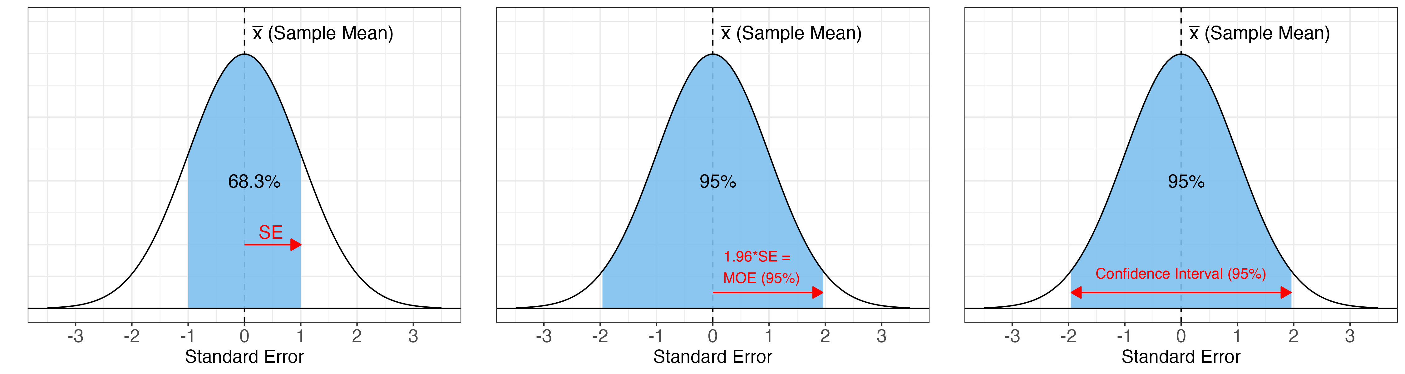
The standard error isn’t super useful by itself. However, it can be used to calculate our level of confidence that our sample mean accurately reflects the population mean!
We can do this using the Margin of Error, which measures the distance away from the sample mean within which the “true” population mean most likely falls.
This multiplies the Standard Error (\(SE\)) by a value \(z\), which represents a specific multiple of the standard error from the sample mean.
Likelihood |
Standard Errors from Sample Mean (z) |
|---|---|
80% |
\(\bar{x}\ \pm\) 1.28 \(SE\) |
90% |
\(\bar{x}\ \pm\) 1.645 \(SE\) |
95% |
\(\bar{x}\ \pm\) 1.96 \(SE\) |
99% |
\(\bar{x}\ \pm\) 2.58 \(SE\) |
These multiples are exactly the same as for standard deviations from the population mean!
For example, if we want to be 95% confident that the true population mean is within a particular range of our sample mean, the formula would be:
margin_of_error = 1.96*standard_error

round(margin_of_error, 2)
This means that we can be 95% certain that the “true” population mean (\(\mu\)) is somewhere between 0.46 hours below the sample mean (\(\bar{x} =\) 8.72 hours), and 0.46 hours above the sample mean.
Confidence Intervals#
We can use the Margin of Error to calculate the range of possible values where we are 95% certain the “true” population mean falls. This is also known as the confidence interval
We can do this by adding and subtracting the Margin of Error from the sample mean:
margin_of_error = 1.96*standard_error

sleep_hours_sample_mean = sleep_hours_sample.mean()

lower_bound = sleep_hours_sample_mean - margin_of_error

upper_bound = sleep_hours_sample_mean + margin_of_error

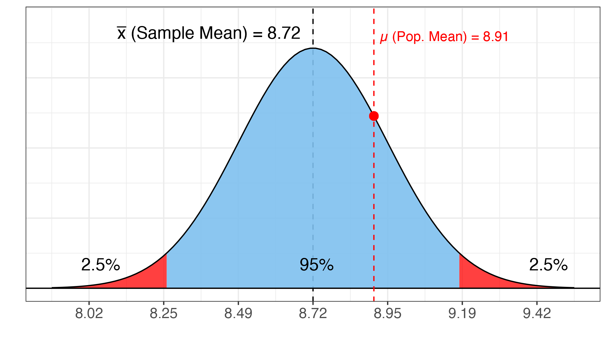
print(f"Based on our sample of 100 people, we are 95% confident that the true population mean is between {round(lower_bound, 2)} and {round(upper_bound, 2)} hours!")
Here is what this test looks like visually - note that our population mean (\(\mu\)) falls within the blue area indicating our range of 95% confidence. This means that at the 95% level, we don’t see any difference between the two means!
If we decrease our confidence level, we can also decrease the size of our confidence interval!
For example, if we only want to be 80% confident, we can lower our multiplier to 1.28. This shrinks our confidence interval.
margin_of_error = 1.28*standard_error

lower_bound = sleep_hours_sample_mean - margin_of_error

upper_bound = sleep_hours_sample_mean + margin_of_error

print(f"Based on our sample of 100 people, we are 80% confident that the true population mean is between {round(lower_bound, 2)} and {round(upper_bound, 2)} hours!")
If we increase our confidence level, we have to increase the size of our confidence interval!
For example, if we only want to be 99% confident, we can increase our multiplier to 2.58.
margin_of_error = 2.58*standard_error

lower_bound = sleep_hours_sample_mean - margin_of_error

upper_bound = sleep_hours_sample_mean + margin_of_error

print(f"Based on our sample of 100 people, we are 99% confident that the true population mean is between {round(lower_bound, 2)} and {round(upper_bound, 2)} hours!")
Hypothesis Testing#
The final step in this process involves answering questions about statistical significance:
Is our sample mean statistically significantly different from the population mean?
In statistics, we ask these types of question by posing two different hypotheses: a default “null” hypothesis where the thing we’re testing is not true, and an “alternative” hypothesis where the thing we’re testing is true. For example:
Is our sample mean statistically significantly different from the population mean?
Null Hypothesis (\(H_0\)): There is no difference between the two means
Alternative Hypothesis (\(H_a\)): There is a difference between the two means
In reality, it is impossible for us to prove or disprove these hypotheses. However, we can attempt to reject the Null Hypothesis.
In other words, we can try to reject the claim that there is no difference between the two means, at a particular level of confidence.
sleep_hours_sample_mean - sleep_hours_mean
Clearly, there is a difference between these two means, or the result of the calculation above would be zero. But is this difference statistically significant?
To determine whether a difference is statistically significant, we need to introduce one more mathematical formula: the t-value. This formula takes the difference between the sample mean and the population mean, and divides that by the standard error (\(\frac{s}{\sqrt{n}}\)):
t_value = (sleep_hours_sample_mean - sleep_hours_mean)/standard_error

t_value
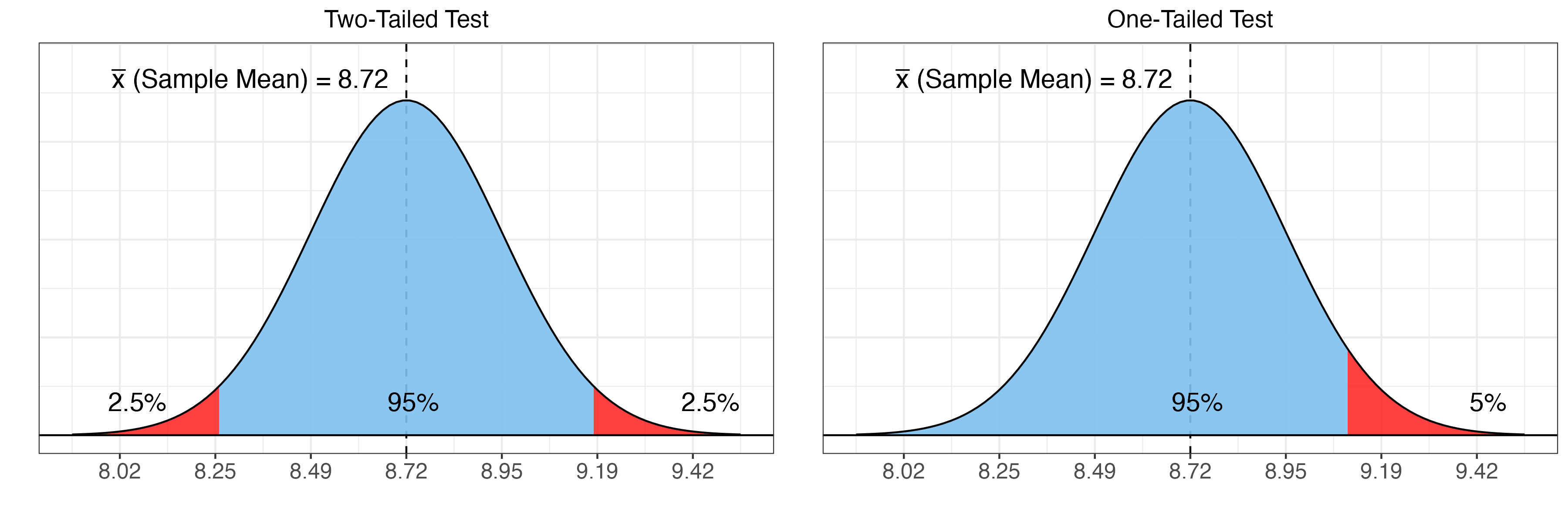
To interpret this value, we must decide whether we are conducting a “one-tailed test” or a “two-tailed test”.
If we are simply interested in whether two values or different, but we don’t care whether the sample mean would be greater than or less than the population mean, then we want a “two-tailed test” looking at both ends of the distribution.
If we have a specific hypothesis about the direction of this relationship - for example, maybe we think that the population mean should be greater than the sample mean – then we want a “one-tailed test” that only looks at one side of the distribution.
Two-Tailed Test#
For a two-tailed test, each value of \(t\) corresponds with a confidence level and a p-value.
Confidence Level (Two-Tailed) |
p-value |
t-value |
|---|---|---|
80% |
20% |
1.28 |
90% |
10% |
1.645 |
95% |
5% |
1.96 |
99% |
1% |
2.58 |
For example, if the absolute value of \(t\) (removing the negative sign) is greater than 1.28:
We are 80% confident that we can reject the Null Hypothesis (that the sample mean is the same as the population mean).
This means that there is still a 20% likelihood that the Null Hypothesis is true (and the means are the same). This is the p-value.
We can’t know the specific likelihood associated with a particular value of \(t\) off the top of our heads (the formula is pretty complicated).
However, there is a function called t.sf in the scipy.stats package, which can help us calculate the p-value!
This function requires that we provide the absolute value of our t-value (using
abs())It also requires “degrees of freedom”, which is \(n - 1\) (in this case, 99). This only really matters for really small samples (under 30), because the numbers are pretty much the same for samples larger than 30.
Finally, because we are conducting a two-tailed test, we need to multiply this value by 2
from scipy.stats import t

p_value = t.sf(abs(t_value), 99)*2

round(p_value, 3)
A p-value of 0.428 means that if the Null Hypothesis is true, there would be a 42.8% likelihood of getting a sample mean at least this far away (0.185 hours) from the population mean.
42.8% is pretty likely, so we cannot reject the Null Hypothesis.
Generally speaking, we should only reject the Null Hypothesis if the p-value is less than 0.05 (or ideally, less than 0.01).
If we had gotten a p-value of 0.05, it would indicate that there would only be a 5% chance of getting a sample mean at least 0.185 hours from the population mean if the Null Hypothesis were true.
One-Tailed Test#
Let’s say instead we wanted to conduct a one-tailed test with the following question
Is our sample mean statistically significantly less than the population mean?
Null Hypothesis (\(H_0\)): The sample mean is greater than or equal to the population mean
Alternative Hypothesis (\(H_a\)): The sample mean is less than the population mean
The only difference with this test is that the likelihood associated with each t-value has changed:
Likelihood (Two-Tailed) |
t-value |
|---|---|
90% |
1.28 |
95% |
1.645 |
97.5% |
1.96 |
99.5% |
2.58 |
For example, ff the absolute value of \(t\) (removing the negative sign) is greater than 1.28:
We are 90% confident (instead of 80%) that we can reject the Null Hypothesis (that the sample mean is the same as the population mean).
This means that there is still a 10% likelihood (instead of 20%) that the Null Hypothesis is true (and the means are the same).
To find the p-value for a one-tailed test, we simply calculate the p-value without multiplying it by 2!
p_value = t.sf(abs(t_value), 99)

round(p_value, 3)
A p-value of 0.214 means that if the Null Hypothesis is true, there would be a 21.4% likelihood of getting a sample mean at least 0.185 hours less than the population mean.
21.4% is still too likely, so we cannot reject the Null Hypothesis; we need a value less than 5%!
Summary#
Population Statistics
Sample Statistics
Standard Error, Margin of Error, and Confidence Interval
t-value