Lecture 9: Statistical Analysis

Lecture 9: Statistical Analysis#

Data Preparation#

import pandas as pd

housing_data = pd.read_excel("housing_dwellings_Toronto_2021_7.xlsx", sheet_name = "Dwelling Characteristics", header = 9)

housing_data.head()

import geopandas as gpd

neighbourhoods = gpd.read_file("Neighbourhoods.geojson")

neighbourhoods.head()

neighbourhood_data = pd.merge(neighbourhoods, housing_data, left_on = ["AREA_NAME"], right_on = ["Neighbourhood Name"])

neighbourhood_data.head()

important_columns = ["AREA_NAME", "CLASSIFICATION", "Single-detached house (%)", "Apartment in a building that has five or more storeys (%)"]

neighbourhood_data = neighbourhood_data[important_columns]

neighbourhood_data

new_column_names = {
    "AREA_NAME": "Neighbourhood",
    "CLASSIFICATION": "Category",
    "Single-detached house (%)": "SFH_share",
    "Apartment in a building that has five or more storeys (%)": "big_apartment_share"
}

neighbourhood_data = neighbourhood_data.rename(columns = new_column_names)

neighbourhood_data

Review: Statistical Inference#

Last time, we discussed methods to determine the likelihood that the mean from a sample is representative of the “true” mean of the overall population that sample is drawn from.

Let’s start by calculating the population mean and standard deviation!

import statistics

single_family = neighbourhood_data["SFH_share"]

population_mean = single_family.mean()

population_sd = statistics.pstdev(single_family) # .pstdev() for *population* standard deviation

print(f"Population Mean = {round(population_mean, 2)}")
print(f"Population Standard Deviation = {round(population_sd, 2)}")

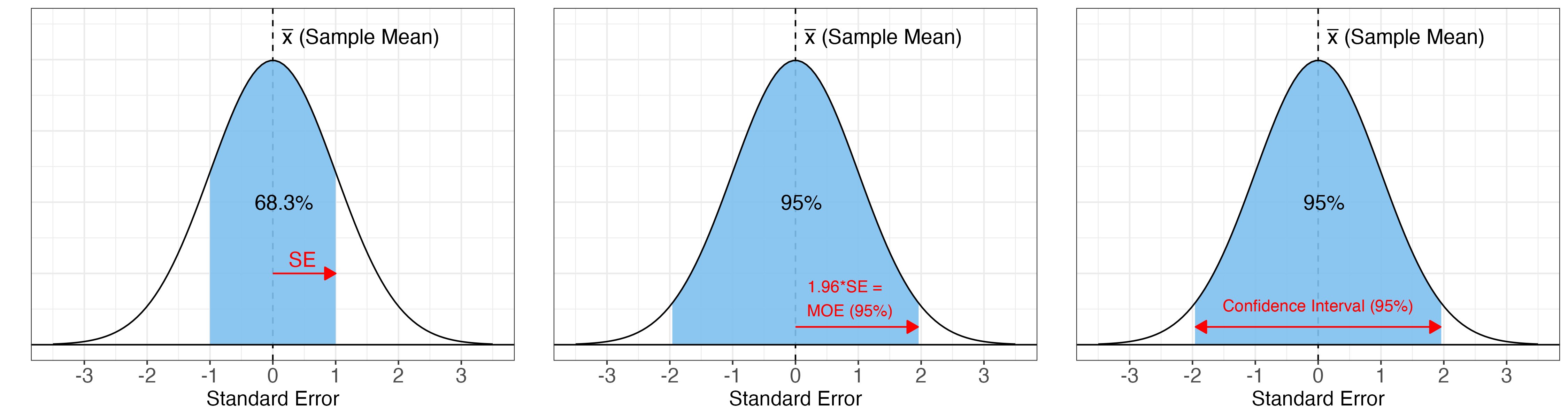
Once again, we can create a random sample and calculate our sample statistics (sample mean and sample standard deviation, as well as standard error, margin of error, and confidence interval).

Standard Error: $SE = s/\sqrt{n}$
Margin of Error: $MOE = z*SE$, where $z$ is a specific value based on our chosen level of confidence
Confidence Interval: $CI = \bar{x} \pm MOE$

sample = single_family.sample(n = 30, replace = False, random_state=1234)

sample_n = len(sample)                      # Sample size

sample_mean = sample.mean()                 # Sample mean
sample_sd = sample.std()                    # .std() for *Sample* Standard Deviation

sample_se = sample_sd/(sample_n**0.5)       # Standard Error
sample_moe = 1.96 * sample_se               # Margin of Error, using 1.96 for 95% confidence level

ci_lower_bound = sample_mean - sample_moe   # Lower bound of confidence interval
ci_upper_bound = sample_mean + sample_moe   # Upper bound of confidence interval

print(f"Sample Size = {sample_n}")
print(f"Sample Mean = {round(sample_mean, 2)}")
print(f"Sample Standard Deviation = {round(sample_sd, 2)}")
print(f"Standard Error = {round(sample_se, 2)}")
print(f"Margin of Error = {round(sample_moe, 2)}")
print(f"Confidence Interval = [{round(ci_lower_bound, 2)}, {round(ci_upper_bound, 2)}]")    

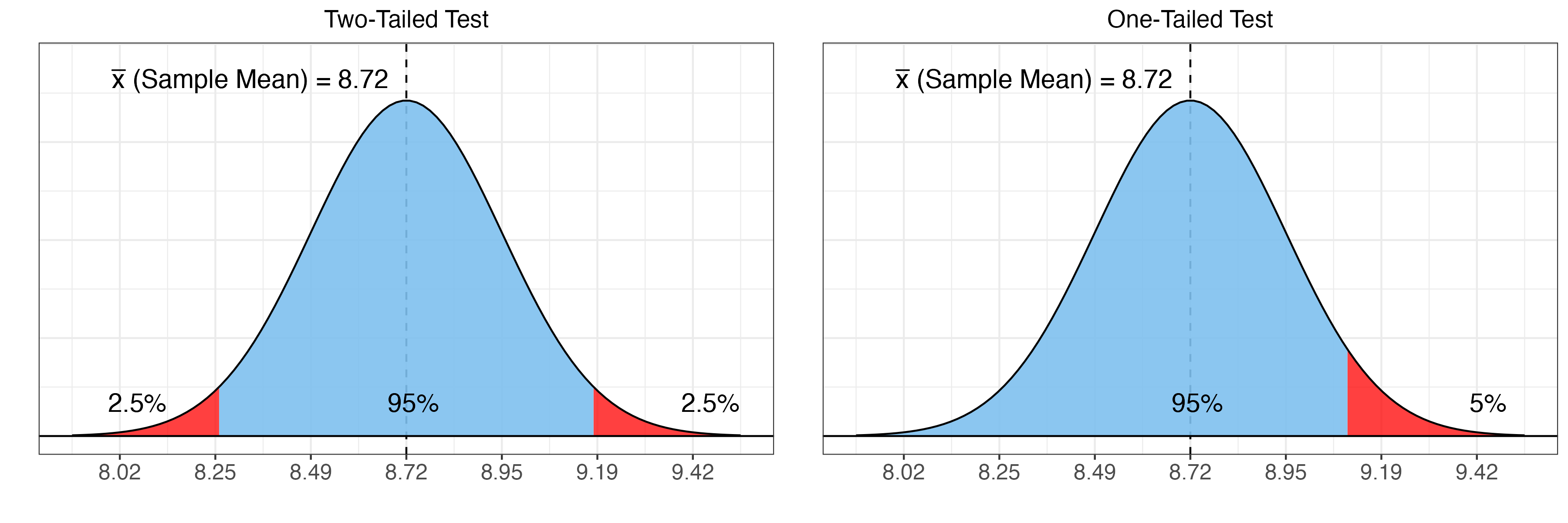
We also talked about hypothesis testing, to determine whether a difference between the sample mean and population mean is statistically significant.

Two-Tailed: Is our sample mean statistically significantly different than the population mean?
- Null Hypothesis ($H_0$): The sample mean is equal to the population mean
- Alternative Hypothesis ($H_a$): The sample mean is different from the population mean
One-Tailed: Is our sample mean statistically significantly greater than (less than) the population mean?
- Null Hypothesis ($H_0$): The sample mean is not greater than (less than) the population mean
- Alternative Hypothesis ($H_a$): The sample mean is greater than (less than) than the population mean

We can test whether to reject the Null Hypothesis by calculating a “t-statistic”:

\[ t = \frac{\bar{x}-\mu}{SE} \]

Then, we compare the value of that t-statistic to this table:

t-value	Confidence Level (2-tail)	p-value (2-tail)	Confidence Level (1-tail)	p-value (1-tail)
1.28	80%	20%	90%	10%
1.645	90%	10%	95%	5%
1.96	95%	5%	97.5%	2.5%
2.58	99%	1%	99.5%	0.5%

The confidence level indicates how confident we want to be that the two means are different.
The p-value indicates the probability that we are wrong, and the Null Hypothesis is true.

t_value = (sample_mean - population_mean)/sample_se

t_value

Rather than calculating this manually every time, we can also use the function ttest_1samp from scipy, which does these calculations automatically. We just need to provide our sample and the population mean.

from scipy import stats

t_test_one_sample = stats.ttest_1samp(sample, popmean = population_mean)

print(t_test_one_sample.statistic)
print(t_test_one_sample.pvalue)

As a reminder, the p-value tells us the probability that our sample mean would be this different from the population mean by chance. A high p-value indicates this sample is very similar to the overall population!

We can also run a one-tailed test, if we want to assess whether the population mean is specifically larger or smaller than the sample mean, by specifying:

alternative="greater" to test if the population mean is larger than the sample mean
alternative="less" to test if the population mean is smaller than the sample mean

t_test_one_sample_one_tail = stats.ttest_1samp(sample, popmean = population_mean, alternative = "greater")

print(t_test_one_sample_one_tail.statistic)
print(t_test_one_sample_one_tail.pvalue)

The t-statistic remains the same but the p-value is smaller, because we are only looking in one direction, so there is a greater chance of ending up in the red zone.

Two-Sample Hypothesis Test#

Instead of testing whether a sample mean is different from a population mean, we can also test whether two samples are different from one another. Two-sample hypothesis tests are super useful for answering statistical questions. For example, our data contains different categories of neighbourhoods defined by the city: “Neighbourhood Improvement Areas”, “Emerging Neighbourhoods”, and other neighbourhoods.

neighbourhood_data.value_counts("Category")

What if we want to compare whether the characteristics of “Neighbourhood Improvement Areas” are different from the rest? Let’s create two samples:

sample1 = “Neighbourhood Improvement Area”
sample2 = All other neighbourhoods

sample1 = neighbourhood_data[neighbourhood_data["Category"] == "Neighbourhood Improvement Area"]["big_apartment_share"]

sample2 = neighbourhood_data[neighbourhood_data["Category"] != "Neighbourhood Improvement Area"]["big_apartment_share"]

print(len(sample1))
print(len(sample2))

Our first sample (of Neighbourhood Improvement Areas) has 33 observations, and our second sample (of all others) has 125 observations.

We can calculate the difference in sample means manually (although the formula is a bit more complex):

\[ t = \frac{\bar{x}_1 - \bar{x}_2}{\sqrt{{\frac{s_1^2}{n_1}} + {\frac{s_2^2}{n_2}}}} \]

sample1_mean = sample1.mean()
sample2_mean = sample2.mean()

sample1_sd = sample1.std()
sample2_sd = sample2.std()

sample1_n = len(sample1)
sample2_n = len(sample2)

t_value = (sample1_mean - sample2_mean)/(((sample1_sd**2/sample1_n) + (sample2_sd**2/sample2_n))**0.5)

print(t_value)

This t-statistic indicates that the % apartments in taller buildings is statistically different in the first sample (NIA neighbourhoods) than in the second sample at a 95% level of confidence.

We can say this because the magnitude of the t-statistic is greater than 1.96 (indicating a 95% confidence level) but lower than 2.58 (indicating a 99% confidence level).

t-value	Confidence Level (2-tail)	p-value (2-tail)
1.28	80%	20%
1.645	90%	10%
1.96	95%	5%
2.58	99%	1%

Rather than having you calculate that formula manually every time, we can use the stats.ttest_ind() function from scipy to run a two-sample difference test.

We are setting equal_var=False, because the variance (how far spread out the values are) is likely to be different between these two samples

from scipy import stats

t_test_two_sample = stats.ttest_ind(sample1, sample2, equal_var=False)

print(t_test_two_sample.statistic)
print(t_test_two_sample.pvalue)

A p-value of 0.0355 indicates that there is only a 3.55% likelihood that the distance between the two means would be more extreme if the Null Hypothesis were true. That’s pretty good, and suggests we can be pretty confident in rejecting the Null Hypothesis!

If we specifically want to ask whether Neighbourhood Improvement Areas (sample1) have more tall apartment buildings than other neighbourhoods (sample2), we can specify alternative='greater', resulting in an even lower p-value!

t_test_two_sample_one_tail = stats.ttest_ind(sample1, sample2, equal_var=False, alternative='greater')

print(t_test_two_sample_one_tail.statistic)
print(t_test_two_sample_one_tail.pvalue)

This test is really powerful, because we can use it to determine whether any two groups are different from one another!

Are lower-income neighbourhoods more likely to exhibit certain health conditions?
Are neighbourhoods with more apartments likely to have smaller household sizes?
And so on!

Correlation#

Another powerful form of statistical analysis is to look at the direct relationship between two different variables. The easiest way to accomplish this is via the calculation of a correlation statistic.

As an example, let’s plot the relationship between the share of tall apartment buildings and the share of detached single-family houses. For bivariate (aka two-variable) visualizations, we will use a scatterplot

neighbourhood_data.plot.scatter("SFH_share", "big_apartment_share")

What do we observe about this relationship?

To quantify how closely related these two variables are, we can use something called a Pearson correlation coefficient (r).

This coefficient is calculated by determining the covariance between the two variables, which calculates the extent to which the two variables vary in the same direction (positive) or opposite directions (negative)
- If values of $x_i$ and $y_i$ tend to be larger/smaller than their averages at the same time, there will be a positive covariance.
- If values of $x_i$ and $y_i$ tend to move in opposite directions ($x_i$ is small when $y_i$ is large and vice versa), there will be a negative covariance.
This covariance is divided by the standard deviations of the two variables ($\sigma_x * \sigma_y$)

\[ r = \frac{cov(x, y)}{\sigma_x*\sigma_y} \quad \quad \quad \quad cov(x, y) = \frac{\Sigma{(x_i - \bar{x})(y_i - \bar{y})}}{n - 1} \]

x = neighbourhood_data["SFH_share"]
y = neighbourhood_data["big_apartment_share"]
n = len(neighbourhood_data)

x_diff = x - x.mean()
y_diff = y - y.mean()

diff_product = x_diff*y_diff

pd.concat([x_diff, y_diff, diff_product], axis = 1, keys = ["x_diff", "y_diff", "diff_product"]) # Create a table showing differences above/below the mean

To calculate the correlation, we can multiply these differences to get the covariance.

We then divide the covariance by the standard deviations to normalize this number, turning it into a value between -1 (where the covariance is as negative as possible) and +1 (where the covariance is as positive as possible). This is the correlation coefficient (r)!

cov_xy = sum(x_diff*y_diff)/(n - 1)

r = cov_xy/(x.std()*y.std())

r

Instead of doing this manually each time, we can use the correlation function from the statistics library to save us the trouble!

import statistics

statistics.correlation(x, y)

Pearson correlation coefficients always range between -1 and +1.

-1 indicates that the data are perfectly negatively correlated (values are in a downward pointing line)
+1 indicates that the data are perefectly positively correlated (values are in an upward pointing line)
0 indicates that there is no relationship between the variables at all!

An example of a perfect correlation is the conversion between two different units, such as temperatures in Celsius and Fahrenheit:

temperature = pd.read_csv("temps.csv")

temperature.plot.scatter("Mean Temp (C)", "Mean Temp (F)")

round(statistics.correlation(temperature["Mean Temp (C)"], temperature["Mean Temp (F)"]), 2)

Linear Regression#

Correlation is useful for telling us that a positive (or negative) relationship exists. For example, we know that there is a negative relationship between single-family homes and tall apartments.
However, this doesn’t tell us directly how one variable affects another. For example, to what extent does an increase in the percentage of single-family homes decrease the percentage of tall apartments?
What we want to do is create a single line (often called the “line of best fit”) that best represents the linear relationship between these two variables.

The formula for a line is:

\[ y = \alpha + \beta{x} \]

Where:

$y$ is the dependent variable: the outcome variable, appearing on the y-axis
$x$ is the independent variable: the input variable, appearing on the x-axis
$\alpha$ is the y-intercept: the point at which $x$ is 0, where the line reaches the y (vertical) axis
$\beta$ is the slope: how steep (or shallow) the line is

We can begin by calculating the slope ($\beta$). This is determined by the relationship between a change in $y$ (fahrenheit) vs a change in $x$ (celsius).

For example, when we observe an increase from 0˚C to 1˚C, we observe an increase from 32˚F to 33.8˚F.
For a change of +1˚C, we have a change of +1.8˚F! Therefore, the slope of the line is $y/x = 1.8/1 = 1.8$.

To calculate $\alpha$, we need to know what the value of $y$ (fahrenheit) would be when $x$ (celsius) $= 0$.

In this case, when it is 0˚C, we know that it will be 32˚F. Therefore, the value of $\alpha$ is 32!

We can now fill in our formula, changing $y$ to $f$ (for fahrenheit) and $x$ to $c$ (for celcius):

\[ y = \alpha + \beta{x} \]

\[ f = 32 + 1.8{c} \]

If we put in any value for $c$ (temperature in celsius), this formula will return $f$ (tempreature in fahrenheit)!

c = 0

f = 32 + 1.8 * c

print(f)

We can also produce outputs for a range for different inputs. For example, we could provide temperatures in celsius between -15 and +35, and get the function to return values in fahrenheit at each temperature.

c = pd.Series(range(-15, 35))

f = 32 + 1.8 * c

f.head()

If we add these values for c and f to our graph as a red line, we can see that it lines up perfectly with the data!

temperature.plot.scatter("Mean Temp (C)", "Mean Temp (F)").plot(c, f, color = "red")

For data that aren’t perfectly correlated, this is a bit more complicated. We can’t just look at two sets of values and know exactly where the line should be, because the actual data are scattered around!

neighbourhood_data.plot.scatter("SFH_share", "big_apartment_share")

Instead of finding a line that perfectly fits the data, our goal is to find a line that best approximates the data, by minimizing its “residual” distance away from each of the individual points (the vertical grey lines in the example image below):

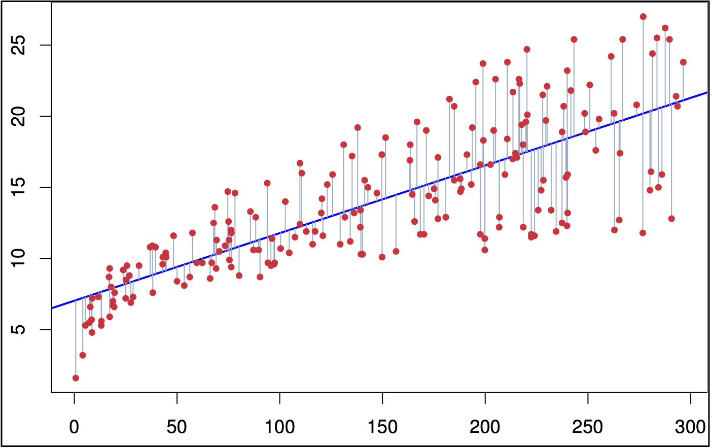
There are a couple of different ways to arrive at the slope of this line. One solution is to take correlation between $x$ and $y$ we calculated earlier ($r$), which tells us the strength and direction of the relationship between the two variables.

We then multiply this by the relationship between the standard deviations of $y$ vs. $x$, which tell us the extent to which $y$ is more or less spread out than $x$:

\[ \beta = r*\frac{\sigma_y}{\sigma_x} \]

slope = (r*(y.std()/x.std()))

print(slope)

To find the intercept ($\alpha$), we find out what its value would be if $y$ and $x$ were both at their average (mean) values:

\[ \alpha = \bar{y} - \beta{\bar{x}} \]

\[ \alpha = \bar{y} - (-0.86{\bar{x}}) \]

intercept = y.mean() - slope*x.mean()

intercept

We now have our formula: $$ y = 63.92 + (- 0.86*x) $$

We can calculate what values of $y$ this formula predicts for each value of $x$, and add these predictions as a new column in our data frame!

predicted_y = intercept + (slope * x)

neighbourhood_data["predicted_apartment_share"] = predicted_y

neighbourhood_data[["SFH_share", "big_apartment_share", "predicted_apartment_share"]]

Now, we’re ready to plot our line, using the original x and the predicted_y produced by our regression formula!

neighbourhood_data.plot.scatter("SFH_share", "big_apartment_share").plot(x, predicted_y, color = "red")

Instead of calculating the slope and intercept manually, we can use the function ols from the statsmodels.formula.api library

from statsmodels.formula.api import ols

model = ols('big_apartment_share ~ SFH_share', data = neighbourhood_data).fit()

print(model.params)

The syntax in the function ols function 'y ~ x' is a special syntax for describing statistical models.
The column name to the left of ~ specifies the dependent variable (big_apartment_share)
The column name to the right of ~ specifies the independent variable(s) (SFH_share).
.fit() at the end tells it to actually run the model
.params can be used to get the intercept and slope!

If we want a full report of the model results, we can use the function .summary() on our model:

print(model.summary())

There’s a lot going on in that table! Let’s pull out the most important information:

model.summary().tables[1]

An Intercept coefficient of 63.92 means that when the share of single-family homes (SFH_share) is 0%, the share of large apartments will be 63.92%.
A coefficient of -0.86 for SFH_share indicates that for each percentage point increase in SFH_share, the percentage of large apartments will decrease by 0.86 points.
- If SFH_share = 1%, the share of large apartments would be $63.92 - (0.86*1) = 63.06\%$
- If SFH_share = 50%, the share of large apartments would be $63.92 - (0.86*50) = 20.92\%$

In addition to the values for the Intercept and the slope (named SFH_share), this summary also reports a standard error (std err), a t value, and several other important pieces of information!

For the slope (SFH_share), the t-value is testing whether the value of the slope is signficantly different from zero (a flat line).
This similarly relies on an assumed normal distribution:

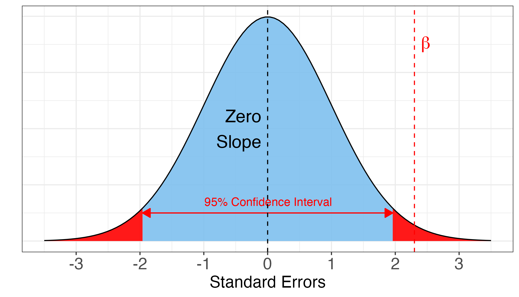
The formula for standard error is a bit more complex than what we have shown so far, but the rest of the statistics can be interpreted the same as for the difference tests:
- t indicates the t-statistic, how many standard errors our estimate is away from zero: $t = \beta/SE = -0.86/0.082 = -10.486$
- P>|t| is the p-value, indicating the probability that our coefficient would be this far away from zero by random chance
- [0.025 0.975] report the 95% confidence interval. We are 95% confident that the slope is somewhere between -1.025 and -0.7

Finally, we can also use this model to determine how much of the variation in our dependent variable (% of units in large apartment buildings) can be explained by our independent variable (% of single-family homes). This value is called “R-squared”.

\[ R^2 = \frac{Regression\ Sum\ of\ Squares\ (RSS)}{Total\ Sum\ of\ Squares\ (TSS)} = \frac{\Sigma{(\hat{y_i}-\bar{y})^2}}{\Sigma{({y_i}-\bar{y})^2}} \]

$\hat{y_i} - \bar{y}$ is the difference between the predicted values for y (based on the line of best fit) and the mean
$y_i - \bar{y}$ is the difference between the actual values for y and the mean.
- In other words, $R^2$ is comparing how well the model predicts values, compared with where the values are actually located

rss = ((predicted_y - y.mean())**2).sum()
tss = ((y - y.mean())**2).sum()

rsquared = rss/tss

print(rsquared)

We can also pull the R-squared directly from the model results!

print(model.rsquared)

This means that the share of single-family homes in a neighbourhood explains 41.3% of the variation in the share of large apartment building units in the neighbourhood.

Relevant “Shortcut” Functions#

One-Sample Hypothesis Tests (sample vs. population): stats.ttest_1samp() (made available by from scipy import stats)
- alternative = "greater" to test if the population mean is greater than the sample mean
- alternative = "less" to test if the population mean is less than the sample mean
Two-Sample Hypothesis Tests: stats.ttest_ind() (made available by from scipy import stats)
- alternative = "greater" to test if the mean of sample1 is greater than the mean of sample2
- alternative = "less" to test if the mean of sample1 is less than the mean of sample2
Correlation: statistics.correlation() (made available by import statistics)
Linear Regression: ols().fit() (made available by from statsmodels.formula.api import ols)
- .params to get the slope and intercept from the model object
- .summary() to obtain the full regression model summary, or .summary().tables[1] to get the coefficient table
- .rsquared to get the r-squared value from the model object