Class 5: Data Transformations, Grouped Data, and Data Visualization

Class 5: Data Transformations, Grouped Data, and Data Visualization#

Last class#

read in a csv file to pandas
select rows and columns from a pandas.DataFrame
rename columns of a pandas.DataFrame

This class#

Transformations: create a new column in a pandas.DataFrame
Data summaries: mean, median, and measures of variation
Data visualization: boxplots, histograms, and bar charts

Midterm Information#

Covers all the content we have covered up until this class.
A past test is available on the course website.
We have set up 2 x 2hr online midterm review sessions (Feb 6 & Feb 7) during which you can ask questions on the practice midterm. We strongly recommend you try the practice midterm before or during the review sessions.
The test was designed to be completed in 90 minutes.
The teaching team will post a link to the test by 09:00 AM, Feb. 11 on the course website.
You can submit anytime up until 11:00 AM on February 11.
The instructors will be available on a zoom link in case you have any questions from 09:00 AM - 11:00 AM. We will also be in the classroom, SS2118 for those who would like to use the space and in-person support.

Data Transformations#

Time in the time use survey is measured in minutes, but it’s not easy to interpret when the numbers get very large.

I worked four thousand six hundred thirty two minutes last week!

It would be easier if time was reported in hours.

I worked over seventy seven hours last week!

Converting time measured in minutes to time measured in hours is an example of a data transformation.

Time use survey#

import pandas as pd

time_use_data = pd.read_csv("gss_tu2016_main_file.csv")

time_use_data.head()

/var/folders/0j/ybsv4ncn5w50v40vdh5jjlww0000gn/T/ipykernel_15264/4239799222.py:1: DeprecationWarning: 
Pyarrow will become a required dependency of pandas in the next major release of pandas (pandas 3.0),
(to allow more performant data types, such as the Arrow string type, and better interoperability with other libraries)
but was not found to be installed on your system.
If this would cause problems for you,
please provide us feedback at https://github.com/pandas-dev/pandas/issues/54466
        
  import pandas as pd

	CASEID	pumfid	wght_per	survmnth	wtbs_001	agecxryg	agegr10	agehsdyc	ageprgrd	chh0014c	...	ree_02	ree_03	rlr_110	lan_01	lanhome	lanhmult	lanmt	lanmtmul	incg1	hhincg1
0	10000	10000	616.6740	7	305.1159	96	5	62	96	0	...	1	1	1	1	1	1	1	1	1	1
1	10001	10001	8516.6140	7	0.0000	6	5	32	5	0	...	5	6	3	1	5	2	5	2	5	8
2	10002	10002	371.7520	1	362.7057	2	4	9	10	3	...	5	1	1	1	1	1	1	1	3	8
3	10003	10003	1019.3135	3	0.0000	96	6	65	96	0	...	3	2	2	1	1	1	1	1	2	2
4	10004	10004	1916.0708	9	11388.9706	96	2	25	96	0	...	9	99	9	9	99	9	99	9	2	4

5 rows × 350 columns

Subset the data#

In this class we will explore the following columns. Let’s create a subset of time_use_data with only these columns:

(columns from last week)

CASEID: participant ID
luc_rst: large urban centre vs rural and small towns
chh0014c: number of kids 14 or under
gtu_110: feeling rushed

(plus…)

prv: province of residence
agegr10: age group
marstat: marital status
sex: sex
dur01: duration spent sleeping
dur08: duration spent working

important_columns = [
    "CASEID", 
    "prv", "luc_rst", # place of residence
    "agegr10", "marstat", "sex", # age, marital status, sex
    "chh0014c", # kids < 14
    "gtu_110", # feeling rushed
    "dur01", "dur08" # time sleeping and working
]

subset_time_use_data = time_use_data[important_columns]

subset_time_use_data.head()

	CASEID	prv	luc_rst	agegr10	marstat	sex	chh0014c	gtu_110	dur01	dur08
0	10000	46	1	5	5	1	0	1	510	0
1	10001	59	1	5	1	1	0	3	420	0
2	10002	47	1	4	1	2	3	1	570	480
3	10003	35	1	6	5	2	0	2	510	20
4	10004	35	1	2	6	1	0	1	525	0

Rename columns so that they are meaningful#

Use the rename function to rename columns.

# dictionary of "old name":"new name"

newnames = {
        "CASEID": "Participant ID",
        "luc_rst": "Urban/Rural",
        "agegr10": "Age Group",
        "marstat": "Marital Status",
        "sex": "sex",
        "chh0014c": "Kids under 14",
        "gtu_110": "Feeling Rushed",
        "dur01": "Sleep duration",
        "dur08": "Work duration"
    }

subset_time_use_data_colnames = subset_time_use_data.rename(columns = newnames)

subset_time_use_data_colnames.head()

	Participant ID	prv	Urban/Rural	Age Group	Marital Status	sex	Kids under 14	Feeling Rushed	Sleep duration	Work duration
0	10000	46	1	5	5	1	0	1	510	0
1	10001	59	1	5	1	1	0	3	420	0
2	10002	47	1	4	1	2	3	1	570	480
3	10003	35	1	6	5	2	0	2	510	20
4	10004	35	1	2	6	1	0	1	525	0

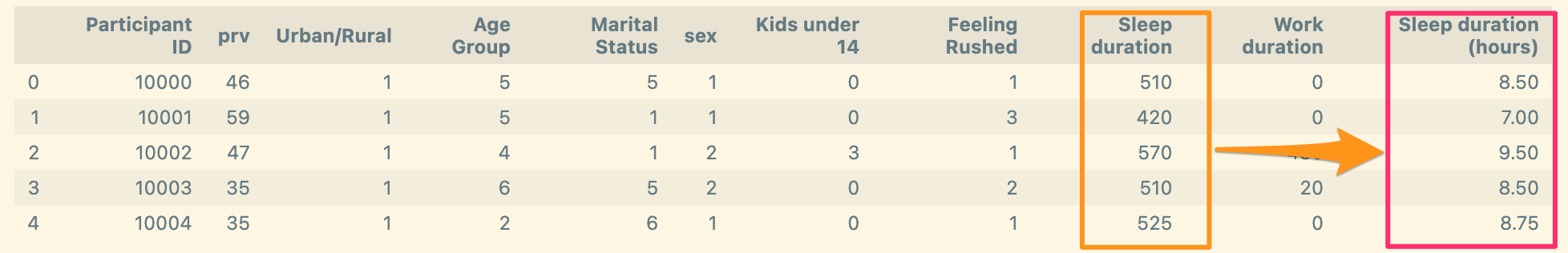
Create a new column in a pandas DataFrame#

Create a new numeric column derived from another numeric column.

The code below creates a new column Sleep duration (hours) by dividing Sleep duration by 60, since 1 hour = 60 minutes.

subset_time_use_data_colnames # create a new column

subset_time_use_data_colnames.head()

	Participant ID	prv	Urban/Rural	Age Group	Marital Status	sex	Kids under 14	Feeling Rushed	Sleep duration	Work duration
0	10000	46	1	5	5	1	0	1	510	0
1	10001	59	1	5	1	1	0	3	420	0
2	10002	47	1	4	1	2	3	1	570	480
3	10003	35	1	6	5	2	0	2	510	20
4	10004	35	1	2	6	1	0	1	525	0

subset_time_use_data_colnames["Sleep duration (hours)"] = subset_time_use_data_colnames["Sleep duration"] / 60

subset_time_use_data_colnames.head()

	Participant ID	prv	Urban/Rural	Age Group	Marital Status	sex	Kids under 14	Feeling Rushed	Sleep duration	Work duration	Sleep duration (hours)
0	10000	46	1	5	5	1	0	1	510	0	8.50
1	10001	59	1	5	1	1	0	3	420	0	7.00
2	10002	47	1	4	1	2	3	1	570	480	9.50
3	10003	35	1	6	5	2	0	2	510	20	8.50
4	10004	35	1	2	6	1	0	1	525	0	8.75

What happened?#

To create a new column, use the [] brackets with the new column name at the left side of the assignment.

The calculation of the values is done element-wise. This means all values in the given column are divided by the value 60 at once. You do not need to use a loop to iterate each of the rows!

Reference is available here.

Transform a column using if-then#

The Age Group column has the following distribution.

subset_time_use_data_colnames["Age Group"].value_counts()

Age Group
  3741
  2958
  2789
  2597
  2127
  1875
  1303
Name: count, dtype: int64

It would be easier to interpret if the labels were used.

           Age group of respondent (groups of 10)

       VALUE  LABEL
           1  15 to 24 years
           2  25 to 34 years
           3  35 to 44 years
           4  45 to 54 years
           5  55 to 64 years
           6  65 to 74 years
           7  75 years and over
          96  Valid skip
          97  Don't know
          98  Refusal
          99  Not stated

       Data type: numeric
       Missing-data codes: 96-99
       Record/column: 1/35

age_group_1 = subset_time_use_data_colnames["Age Group"] == 1
subset_time_use_data_colnames[age_group_1]
subset_time_use_data_colnames.loc[age_group_1, ["Age Group"]]

	Age Group
5	1
6	1
27	1
54	1
59	1
...	...
17341	1
17357	1
17374	1
17378	1
17385	1

1303 rows × 1 columns

# make a copy of the dataframe
subset_time_df = subset_time_use_data_colnames.copy()

# create a new column called "Age group label"

subset_time_df.loc[subset_time_df["Age Group"] == 1, "Age group label"] = "15-24"

subset_time_df.loc[subset_time_df["Age Group"] == 2, "Age group label"] = "25-34"

subset_time_df.loc[subset_time_df["Age Group"] == 3, "Age group label"] = "35-44"

subset_time_df.loc[subset_time_df["Age Group"] == 4, "Age group label"] = "45-54"

subset_time_df.loc[subset_time_df["Age Group"] == 5, "Age group label"] = "55-64"

subset_time_df.loc[subset_time_df["Age Group"] == 6, "Age group label"] = "65-74"

subset_time_df.loc[subset_time_df["Age Group"] == 7, "Age group label"] = "75+"

subset_time_df.head()

	Participant ID	prv	Urban/Rural	Age Group	Marital Status	sex	Kids under 14	Feeling Rushed	Sleep duration	Work duration	Sleep duration (hours)	Age group label
0	10000	46	1	5	5	1	0	1	510	0	8.50	55-64
1	10001	59	1	5	1	1	0	3	420	0	7.00	55-64
2	10002	47	1	4	1	2	3	1	570	480	9.50	45-54
3	10003	35	1	6	5	2	0	2	510	20	8.50	65-74
4	10004	35	1	2	6	1	0	1	525	0	8.75	25-34

What happened?#

To create a new column in a pandas DataFrame using if-then/if-then-else logic#

This line

`subset_time_df.loc[subset_time_df[“Age Group”] == 1, “Age group label”] = “15-24”

creates a new column in subset_time_df called Age group label according to the if-then (conditional) logic:

If subset_time_df["Age Group"] == 1 then Age group label is assigned the value 15-24.

This line

subset_time_df.loc[subset_time_df["Age Group"] == 2, 'Age group label'] = "25-34"

does the else if logic. Namely,

If subset_time_df["Age Group"] == 2 then Age group label is assigned the value 25-34.

This line

subset_time_df.loc[subset_time_df["Age Group"] == 3, "Age group label"] = "35-44"

does the else if logic. Namely,

If subset_time_df["Age Group"] == 3 then Age group label is assigned the value 35-44.

etc …

See idioms in the Pandas cookbook and a reference on different ways to subset a pandas DataFrame.

Merging pandas DataFrames#

We want would like to look at the relationship between sleeping and working, on different aspects of time use at the provincial level. In addition we would like to add provincial level data of on income and housing.
The data is in provincial_data.csv.

prov_data = pd.read_csv("provincial_data.csv")
prov_data

	COL0	COL1	COL2	COL3	COL4
0	1	60.2	70336.0	2.4	16.6
1	10	49.5	67272.0	2.3	10.6
2	11	58.2	61163.0	2.3	11.1
3	12	55.2	60764.0	2.3	12.0
4	13	54.6	59347.0	2.3	10.3
5	24	59.5	59822.0	2.3	12.9
6	35	59.9	74287.0	2.6	19.8
7	46	61.7	68147.0	2.5	11.4
8	47	63.5	75412.0	2.5	12.1
9	48	65.4	93835.0	2.6	15.1
10	59	59.6	69995.0	2.4	20.7
11	60	68.5	84521.0	2.3	12.7
12	61	66.2	117688.0	2.7	9.0
13	62	53.6	97441.0	3.6	7.9

COL0 - GEO UID
COL1 - Labour - Total Sex / Employment rate
COL2 - Income - Total Sex / Total - Income statistics in 2015 for private households by household size - 100% data / Median total income of households in 2015 ($)
COL3 - Dwelling characteristics / Average household size

COL4 - Housing - Total Sex / Total - Owner households in non-farm, non-reserve private dwellings - 25% sample data / % of owner households spending 30% or more of its income on shelter costs

Let’s give the columns meaningful names.

colnames = {"COL0": "Prov", 
            "COL1": "Employment Rate", 
            "COL2": "Income",
            "COL3": "Household Size",
            "COL4": "Pct house over 30"}

prov_data.rename(columns=colnames, inplace=True)
# inplace=True applies the column name change to the current DataFrame
prov_data

	Prov	Employment Rate	Income	Household Size	Pct house over 30
0	1	60.2	70336.0	2.4	16.6
1	10	49.5	67272.0	2.3	10.6
2	11	58.2	61163.0	2.3	11.1
3	12	55.2	60764.0	2.3	12.0
4	13	54.6	59347.0	2.3	10.3
5	24	59.5	59822.0	2.3	12.9
6	35	59.9	74287.0	2.6	19.8
7	46	61.7	68147.0	2.5	11.4
8	47	63.5	75412.0	2.5	12.1
9	48	65.4	93835.0	2.6	15.1
10	59	59.6	69995.0	2.4	20.7
11	60	68.5	84521.0	2.3	12.7
12	61	66.2	117688.0	2.7	9.0
13	62	53.6	97441.0	3.6	7.9

Now, we are ready to use the merge function in pandas.

prov_data_df = subset_time_df.merge(
    prov_data, 
    right_on="Prov", # the right data frame is prov_data 
    left_on="prv"    # the left data frame is subset_time_df
)   

prov_data_df.head()

	Participant ID	prv	Urban/Rural	Age Group	Marital Status	sex	Kids under 14	Feeling Rushed	Sleep duration	Work duration	Sleep duration (hours)	Age group label	Prov	Employment Rate	Income	Household Size	Pct house over 30
0	10000	46	1	5	5	1	0	1	510	0	8.50	55-64	46	61.7	68147.0	2.5	11.4
1	10001	59	1	5	1	1	0	3	420	0	7.00	55-64	59	59.6	69995.0	2.4	20.7
2	10002	47	1	4	1	2	3	1	570	480	9.50	45-54	47	63.5	75412.0	2.5	12.1
3	10003	35	1	6	5	2	0	2	510	20	8.50	65-74	35	59.9	74287.0	2.6	19.8
4	10004	35	1	2	6	1	0	1	525	0	8.75	25-34	35	59.9	74287.0	2.6	19.8

Is time spent resting different by province?#

Grouped summaries of data#

Many times we will want to calculate means, proportions, and other statistics by group membership.
This is so common that pandas has a built-in function called groupby that groups a data frame by another variable.

prov_data_df.head()

	Participant ID	prv	Urban/Rural	Age Group	Marital Status	sex	Kids under 14	Feeling Rushed	Sleep duration	Work duration	Sleep duration (hours)	Age group label	Prov	Employment Rate	Income	Household Size	Pct house over 30
0	10000	46	1	5	5	1	0	1	510	0	8.50	55-64	46	61.7	68147.0	2.5	11.4
1	10001	59	1	5	1	1	0	3	420	0	7.00	55-64	59	59.6	69995.0	2.4	20.7
2	10002	47	1	4	1	2	3	1	570	480	9.50	45-54	47	63.5	75412.0	2.5	12.1
3	10003	35	1	6	5	2	0	2	510	20	8.50	65-74	35	59.9	74287.0	2.6	19.8
4	10004	35	1	2	6	1	0	1	525	0	8.75	25-34	35	59.9	74287.0	2.6	19.8

grouped_by_prov = prov_data_df.groupby("Prov") #group the DataFrame by prov

type(grouped_by_prov)

pandas.core.groupby.generic.DataFrameGroupBy

rest_by_prov_mean = grouped_by_prov["Sleep duration (hours)"].mean()

rest_by_prov_mean

Prov
  8.651739
  8.901090
  8.500917
  8.722338
  8.759245
  8.612381
  8.829857
  8.824515
  8.710498
  8.808136
Name: Sleep duration (hours), dtype: float64

rest_by_prov_mean is a pandas Series with indexed by Prov.

type(rest_by_prov_mean)

pandas.core.series.Series

DataFrame Index#

rest_by_prov_mean.index

Index([10, 11, 12, 13, 24, 35, 46, 47, 48, 59], dtype='int64', name='Prov')

From the

  prv                Province of residence

           VALUE  LABEL
              10  Newfoundland and Labroador
              11  Prince Edward Island
              12  Nova Scotia
              13  New Brunswick
              24  Quebec
              35  Ontario
              46  Manitoba
              47  Saskatchewan
              48  Alberta
              59  British Columbia
              96  Valid skip
              97  Don't know
              98  Refusal
              99  Not stated

           Data type: numeric
           Missing-data codes: 96-99
           Record/columns: 1/57-58

We can reindex rest_by_prov_mean.

index_new = [
    "Newfoundland and Labrador", 
    "Prince Edward Island", 
    "Nova Scotia", 
    "New Brunswick",
    "Quebec",
    "Ontario", 
    "Manitoba",
    "Saskatchewan", 
    "Alberta",
    "British Columbia"
]

rest_by_prov_mean.index = index_new

rest_by_prov_mean

Newfoundland and Labrador    8.651739
Prince Edward Island         8.901090
Nova Scotia                  8.500917
New Brunswick                8.722338
Quebec                       8.759245
Ontario                      8.612381
Manitoba                     8.829857
Saskatchewan                 8.824515
Alberta                      8.710498
British Columbia             8.808136
Name: Sleep duration (hours), dtype: float64

Let’s also create a new column Prov label in prov_data_df.

prov_data_df.loc[prov_data_df["Prov"] == 10, "Prov label"] = "NL"

prov_data_df.loc[prov_data_df["Prov"] == 11, "Prov label"] = "Prince Edward Island"

prov_data_df.loc[prov_data_df["Prov"] == 12, "Prov label"] = "Nova Scotia"

prov_data_df.loc[prov_data_df["Prov"] == 13, "Prov label"] = "New Brunswick"

prov_data_df.loc[prov_data_df["Prov"] == 24, "Prov label"] = "Quebec"

prov_data_df.loc[prov_data_df["Prov"] == 35, "Prov label"] = "Ontario"

prov_data_df.loc[prov_data_df["Prov"] == 46, "Prov label"] = "Manitoba"

prov_data_df.loc[prov_data_df["Prov"] == 47, "Prov label"] = "Saskatchewan"

prov_data_df.loc[prov_data_df["Prov"] == 48, "Prov label"] = "Alberta"

prov_data_df.loc[prov_data_df["Prov"] == 59, "Prov label"] = "British Columbia"

prov_data_df.loc[prov_data_df["Prov"] >= 96, "Prov label"] = None

prov_data_df.head()

	Participant ID	prv	Urban/Rural	Age Group	Marital Status	sex	Kids under 14	Feeling Rushed	Sleep duration	Work duration	Sleep duration (hours)	Age group label	Prov	Employment Rate	Income	Household Size	Pct house over 30	Prov label
0	10000	46	1	5	5	1	0	1	510	0	8.50	55-64	46	61.7	68147.0	2.5	11.4	Manitoba
1	10001	59	1	5	1	1	0	3	420	0	7.00	55-64	59	59.6	69995.0	2.4	20.7	British Columbia
2	10002	47	1	4	1	2	3	1	570	480	9.50	45-54	47	63.5	75412.0	2.5	12.1	Saskatchewan
3	10003	35	1	6	5	2	0	2	510	20	8.50	65-74	35	59.9	74287.0	2.6	19.8	Ontario
4	10004	35	1	2	6	1	0	1	525	0	8.75	25-34	35	59.9	74287.0	2.6	19.8	Ontario

Summing across rows of a DataFrame#

How much time is spent by each respondent sleeping and working?

The average time spent sleeping and working by province is:

restwork_by_prov_mean = prov_data_df.groupby("Prov label")[["Sleep duration", "Work duration"]].mean()

restwork_by_prov_mean

	Sleep duration	Work duration
Prov label
Alberta	522.629888	199.491620
British Columbia	528.488161	165.233753
Manitoba	529.791411	175.156442
NL	519.104339	133.946281
New Brunswick	523.340265	148.428166
Nova Scotia	510.055019	158.398649
Ontario	516.742869	177.705566
Prince Edward Island	534.065385	134.126923
Quebec	525.554724	159.450461
Saskatchewan	529.470905	182.572198

Two different ways to calulate row totals#

There are more but we will focus on the two methods.

We would like to calculate the total mean time spent sleeping and working.

restwork_by_prov_mean["Total1"] = restwork_by_prov_mean["Sleep duration"] + restwork_by_prov_mean["Work duration"]

restwork_by_prov_mean.head()

	Sleep duration	Work duration	Total1
Prov label
Alberta	522.629888	199.491620	722.121508
British Columbia	528.488161	165.233753	693.721914
Manitoba	529.791411	175.156442	704.947853
NL	519.104339	133.946281	653.050620
New Brunswick	523.340265	148.428166	671.768431

restwork_by_prov_mean["Total2"] = restwork_by_prov_mean[["Sleep duration","Work duration"]].sum(
    axis=1 # sum across all columns 
)

restwork_by_prov_mean.head()

	Sleep duration	Work duration	Total1	Total2
Prov label
Alberta	522.629888	199.491620	722.121508	722.121508
British Columbia	528.488161	165.233753	693.721914	693.721914
Manitoba	529.791411	175.156442	704.947853	704.947853
NL	519.104339	133.946281	653.050620	653.050620
New Brunswick	523.340265	148.428166	671.768431	671.768431

In pandas axis=1 refers to columns and axis=0 refers to rows.
DataFrame.sum(axis=1): sum across columns
DataFrame.sum(axis=0): sum across rows.

Statistical Variables#

Categorical variable

A categorical variable is a variable for which the measurement scale consists of a set of categories.
For example, time use has ten categories, or levels.
These types of variables are very common in social and biomedical sciences, and many other areas.

Nominal variable

Categorical variables that don't have a natural ordering is called a nominal variable.
For example, Canadian provinces are nominal.

Ordinal variable

If a categorical variable has a natural ordering, it is called an ordinal variable.
For example, if levels 96 (valid skip), 97 (don't know), 98 (refusal), 99 (not stated) are removed from gtu_110 then time use woudl be considered an ordinal variable since it's ordered from feeling rushed Everyday (1) to feeling rushed Never (6).
Ordinal variables clearly order categories, but the "distance" between categories are unknown/meaningless.

Quantitative variable

A quantitative variable consists of numerical measurements.

Interval variable

An interval variable has numerical differences, but there is no relative scale and 0 holds no meaning.
For example, absolute differences between 20℃ and 30℃, and between 10℃ and 20℃ are the same while relative differences between 15℃ and 30℃, and between 10℃ and 20℃ are not.
This is because a 0 value is arbitrary. 0℃ does not mean "no temperature".

An interval variable is one that does have numerical distances between any two levels of the measurement scale. For example, calendar years is an interval variable.

Ratio variable

A ratio variable has both numerical differences and relative scales. A 0 holds semantic meaning.
Time use in minutes and age in years are examples of ratio (statistical) variables.
Time use of 0 minute means no time spent.

What’s the difference between a Statistical Variable and a Variable in python?#

A variable in python is a location in computer memory to store a value.
A statistical variable is essentially a mathematical representation of data.

Examples of implementing statistical variables in python#

If 10 people are randomly selected, and asked how many minutes they slept last night, then this data could be represented by an ratio variable.

In python the data could be represented in pandas.Series, where the Series data type is float.

If 10 people are randomly selected, and asked if they live in urban or rural areas, then this data could be represented by an categorical variable.

In python the data could be represented in pandas.Series, where the Series data type is Boolean (True if urban, and False if not urban).

Statistical Distributions#

What is a statistical distribution?
How can a distribution be summarized?
What questions can we answer using a distribution?

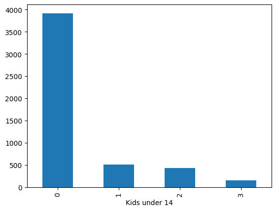
What is the distribution of kids under 14 in Ontario?#

Select rows in prov_data_df where Prov label is Ontario
Select the column Kids under 14
Compute the number of respondents who have 0 kids, 1 kid, etc. using .value_counts()

Ontkidsdist = prov_data_df.loc[
    prov_data_df["Prov label"] == "Ontario",
    "Kids under 14"
].value_counts()

Ontkidsdist

Kids under 14
0    3918
1     508
2     430
3     157
Name: count, dtype: int64

type(Ontkidsdist)

pandas.core.series.Series

A bar plot of the distribution of kids under 14 in Ontario#

Ontkidsdist.plot.bar();

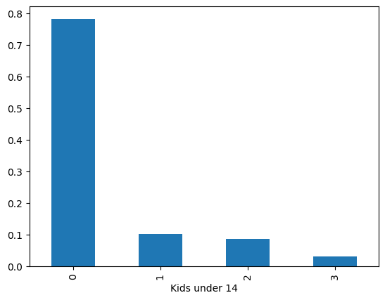
../../../_images/cfde237607e489a1126586f679d32c26f5083aeb4c1161ea3472a0d005a62130.png

If we want to plot proportions instead of counts then we can transform Ontkidsdist by dividing by the total number of observations.

Ontkidsdist_prop = Ontkidsdist / Ontkidsdist.sum()
Ontkidsdist_prop

Kids under 14
0    0.781568
1    0.101337
2    0.085777
3    0.031319
Name: count, dtype: float64

Ontkidsdist_prop.plot.bar();

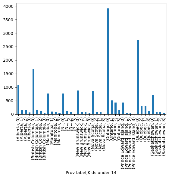
../../../_images/aee9cb1ea4962a8950494826024e6470f0925194f2d31505ab8114576f474a73.png

Distribution of counts by province

prov_data_df.groupby(["Prov label"])["Kids under 14"].value_counts()

Prov label            Kids under 14
Alberta               0                1077
                      1                 152
                      2                 145
                      3                  58
British Columbia      0                1672
                      1                 145
                      2                 132
                      3                  36
Manitoba              0                 763
                      1                  93
                      2                  88
                      3                  34
NL                    0                 766
                      1                 103
                      2                  84
                      3                  15
New Brunswick         0                 875
                      2                  79
                      1                  77
                      3                  27
Nova Scotia           0                 858
                      2                  86
                      1                  77
                      3                  15
Ontario               0                3918
                      1                 508
                      2                 430
                      3                 157
Prince Edward Island  0                 432
                      1                  43
                      2                  30
                      3                  15
Quebec                0                2755
                      2                 305
                      1                 300
                      3                 112
Saskatchewan          0                 716
                      1                  89
                      2                  79
                      3                  44
Name: count, dtype: int64

# an exmaple of a bad plot
prov_data_df.groupby(["Prov label"])["Kids under 14"].value_counts().plot.bar();

../../../_images/599c4f42fad009b9049affbac7a7f8eb157f649821054020f889a0b45e79c3b1.png

# ----- WON'T BE TESTED -----
# the code below is beyond what will be tested and is provided for the purpose 
# of demonstrating examples of visualizations that achieve different goals

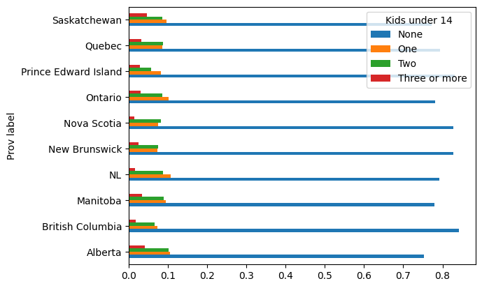
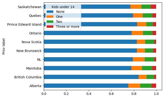
# You can "unstack" the index an create  a better view to achieve different goals.
prov_kids14_dist_df = prov_data_df.groupby(["Prov label"])["Kids under 14"].value_counts()
prov_kids14_dist_unstacked_df = prov_kids14_dist_df.unstack(level=1)

# using "df.plot.barh()" to plot horizontal bars to compari proportions
prov_kids14_totals = prov_kids14_dist_unstacked_df.sum(axis=1)
prov_kids14_dist_unstacked_df["None"] = prov_kids14_dist_unstacked_df[0] / prov_kids14_totals
prov_kids14_dist_unstacked_df["One"] = prov_kids14_dist_unstacked_df[1] / prov_kids14_totals
prov_kids14_dist_unstacked_df["Two"] = prov_kids14_dist_unstacked_df[2] / prov_kids14_totals
prov_kids14_dist_unstacked_df["Three or more"] = prov_kids14_dist_unstacked_df[3] / prov_kids14_totals

## comparing within provinces
prov_kids14_dist_unstacked_df[["None", "One", "Two", "Three or more"]].plot.barh()
## comparing between provinces
prov_kids14_dist_unstacked_df[["None", "One", "Two", "Three or more"]].plot.barh(stacked=True)

<Axes: ylabel='Prov label'>

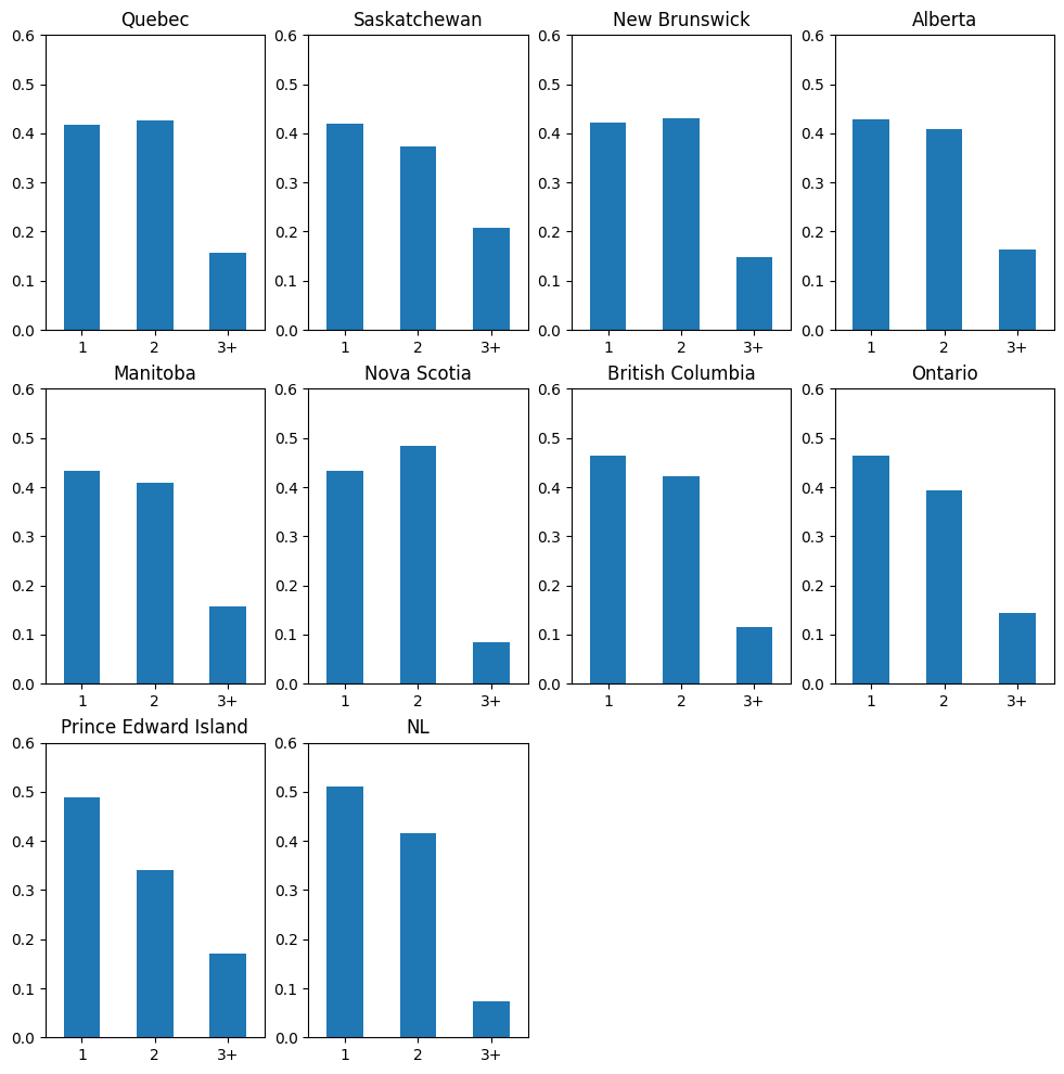
../../../_images/beb8d78debdb6e17975cee1ead1fc3016e2d11d7d8bf7b5bcfa9a75e101444fd.png

../../../_images/478d49e92e777c073525b5fefce179a9e938911e43c748d477ff3ab607d306b4.png

# ----- WON'T BE TESTED -----
# the code below is beyond what will be tested and is provided for the purpose 
# of demonstrating examples of visualizations that achieve different goals

# using "matplotlib" to create "subplots" - will briefly cover in Week 10
# ustack provinces instead of responses
prov_kids14_dist_unstacked_prov_df = prov_kids14_dist_df.unstack(level=0)
prov_kids14_dist_with_ch14_df = prov_kids14_dist_unstacked_prov_df.loc[[1, 2, 3]] # only compare the distribution with 1 or more children
prov_kids14_dist_with_ch14_df = prov_kids14_dist_with_ch14_df / prov_kids14_dist_with_ch14_df.sum(axis=0) # get proportions
# prov_kids14_dist_with_ch14_df.loc[1].sort_values() # check the order by # participants with 1 child < 14

import matplotlib.pyplot as plt
fig, axes = plt.subplots(nrows=3, ncols=4, figsize = (12,12))
# row 1, column 1
ax = axes[0][0]
prov_kids14_dist_with_ch14_df["Quebec"].plot(ax=ax, kind="bar", rot=0)
ax.set_title("Quebec")
ax.set_xticklabels(["1", "2", "3+"])
ax.set_xlabel("")
ax.set_ylim([0, 0.6])

# row 1, column 2
ax = axes[0][1]
prov_kids14_dist_with_ch14_df["Saskatchewan"].plot(ax=ax, kind="bar", rot=0)
ax.set_title("Saskatchewan")
ax.set_xticklabels(["1", "2", "3+"])
ax.set_xlabel("")
ax.set_ylim([0, 0.6])

# row 1, column 3
ax = axes[0][2]
prov_kids14_dist_with_ch14_df["New Brunswick"].plot(ax=ax, kind="bar", rot=0)
ax.set_title("New Brunswick")
ax.set_xticklabels(["1", "2", "3+"])
ax.set_xlabel("")
ax.set_ylim([0, 0.6])

# row 1, column 4
ax = axes[0][3]
prov_kids14_dist_with_ch14_df["Alberta"].plot(ax=ax, kind="bar", rot=0)
ax.set_title("Alberta")
ax.set_xticklabels(["1", "2", "3+"])
ax.set_xlabel("")
ax.set_ylim([0, 0.6])

# row 2, column 1
ax = axes[1][0]
prov_kids14_dist_with_ch14_df["Manitoba"].plot(ax=ax, kind="bar", rot=0)
ax.set_title("Manitoba")
ax.set_xticklabels(["1", "2", "3+"])
ax.set_xlabel("")
ax.set_ylim([0, 0.6])

# row 2, column 2
ax = axes[1][1]
prov_kids14_dist_with_ch14_df["Nova Scotia"].plot(ax=ax, kind="bar", rot=0)
ax.set_title("Nova Scotia")
ax.set_xticklabels(["1", "2", "3+"])
ax.set_xlabel("")
ax.set_ylim([0, 0.6])

# row 2, column 3
ax = axes[1][2]
prov_kids14_dist_with_ch14_df["British Columbia"].plot(ax=ax, kind="bar", rot=0)
ax.set_title("British Columbia")
ax.set_xticklabels(["1", "2", "3+"])
ax.set_xlabel("")
ax.set_ylim([0, 0.6])

# row 2, column 4
ax = axes[1][3]
prov_kids14_dist_with_ch14_df["Ontario"].plot(ax=ax, kind="bar", rot=0)
ax.set_title("Ontario")
ax.set_xticklabels(["1", "2", "3+"])
ax.set_xlabel("")
ax.set_ylim([0, 0.6])

# row 3, column 1
ax = axes[2][0]
prov_kids14_dist_with_ch14_df["Prince Edward Island"].plot(ax=ax, kind="bar", rot=0)
ax.set_title("Prince Edward Island")
ax.set_xticklabels(["1", "2", "3+"])
ax.set_xlabel("")
ax.set_ylim([0, 0.6])

# row 3, column 2
ax = axes[2][1]
prov_kids14_dist_with_ch14_df["NL"].plot(ax=ax, kind="bar", rot=0)
ax.set_title("NL")
ax.set_xticklabels(["1", "2", "3+"])
ax.set_xlabel("")
ax.set_ylim([0, 0.6])

fig.delaxes(axes[2][2])
fig.delaxes(axes[2][3])

../../../_images/7c4ff604c62a768ba68d1da431ffe4f2a7e36764826dba813b759fbbed423fe1.png

Summarizing the distribution of a quantitative variable#

dur01 is time spent sleeping, resting, etc.

dur01              Duration - Sleeping, resting, relaxing, sick in bed

           VALUE  LABEL
               0  No time spent doing this activity
            9996  Valid skip
            9997  Don't know
            9998  Refusal
            9999  Not stated

           Data type: numeric
           Missing-data codes: 9996-9999
           Record/columns: 1/65-68

Sleepduration = prov_data_df["Sleep duration (hours)"]

print(type(Sleepduration))

Sleepduration.dtypes

<class 'pandas.core.series.Series'>

dtype('float64')

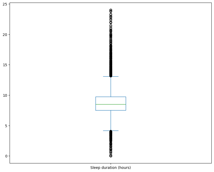
Sleepduration.describe()

count    17390.000000
mean         8.706552
std          2.217733
min          0.000000
25%          7.500000
50%          8.500000
75%          9.750000
max         24.000000
Name: Sleep duration (hours), dtype: float64

The distributions of quantitative variables are often described as:

a measure of centre such as mean, median, and mode
a measure of spread such as standard deviation and inter-quartile range
a measure of range - the largest value minus the smallest value (or max - min)

Quantiles#

The median value is the 50% quantile. 50% of the values fall below this value. The median is also called the second quartile.
The 25% quantile is the value where 25% of the values fall below. This is often the first quartile (Q1)
The 75% quantile is the value where 75% of the values fall below. This is often the third quartile (Q3)
There are 17390 values. If we sort sleep duration values from largest to smallest then find the value in the middle (17390 / 2 = 8695) then that value is the median.

Variation#

One of the most important concepts in statistical reasoning.
Standard deviation is average deviation from the mean. Large values mean large variation and small values mean small variation.
Small samples often have large variation, so estimating a statistic from a small sample is usually less reliable.

Question#

A certain town is served by two hospitals. In the larger hospital about 45 babies are born each day, and in the smaller hospital about 15 babies are born each day. As you know, about 50% of all babies are boys. However, the exact percentage varies from day to day. Sometimes it may be higher than 50%, sometimes lower.

For a period of 1 year, each hospital recorded the days on which more than 60% of the babies born were boys. Which hospital do you think recorded more such days?

The larger hospital
The smaller hospital
About the same (that is, within 5% of each other)

Histograms#

Histograms display the frequency distribution of a quantitative variable.

Sleepduration_hist =  Sleepduration.plot.hist(
    bins=10, 
    edgecolor="black", 
    color="grey", 
    figsize = (8, 6)
);

Sleepduration_hist.set_xlabel("Sleep duration (hours)");

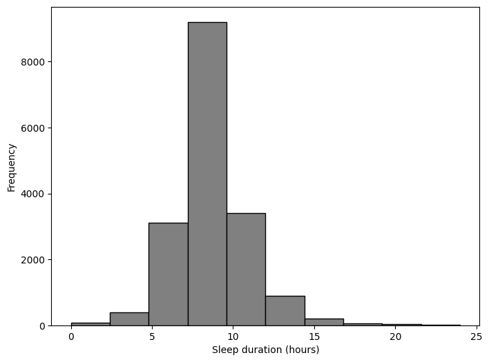
../../../_images/79c602c64e7ba8b0d76c2d6a7b6eb3d69d49b750ca109a64d1912ed349943673.png

pd.cut(Sleepduration, bins=10)

        (7.2, 9.6]
        (4.8, 7.2]
        (7.2, 9.6]
        (7.2, 9.6]
        (7.2, 9.6]
             ...     
    (7.2, 9.6]
   (9.6, 12.0]
    (7.2, 9.6]
  (12.0, 14.4]
    (7.2, 9.6]
Name: Sleep duration (hours), Length: 17390, dtype: category
Categories (10, interval[float64, right]): [(-0.024, 2.4] < (2.4, 4.8] < (4.8, 7.2] < (7.2, 9.6] ... (14.4, 16.8] < (16.8, 19.2] < (19.2, 21.6] < (21.6, 24.0]]

Boxplots#

Another way to visualize the distribution of a quantitative variable
A box plot is a method for graphically depicting groups of numerical data through their quartiles.
The box extends from the Q1 to Q3 quartile values of the data, with a line at the median (Q2).
The whiskers extend from the edges of box to show the range of the data.
By default, they extend no more than 1.5 * IQR (IQR = Q3 - Q1) from the edges of the box, ending at the farthest data point within that interval. Outliers are plotted as separate dots.

Sleepduration_boxplot = Sleepduration.plot.box(figsize = (10,8));

Sleepduration_boxplot;

../../../_images/c128e4d2f28ee5bd81f8184ecf6b8a3d8f5565dc70bb366da52e52023ccffdb3.png

Anatomy of a Boxplot#

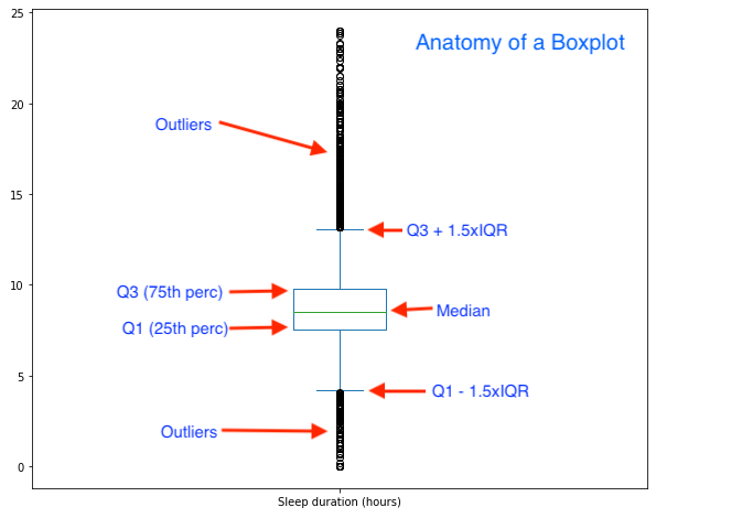
Two pandas methods to create a boxplot are:

pandas.DataFrame.plot.box: plot a Series or columns of a DataFrame
pandas.DataFrame.boxplot: plot the columns of a DataFrame with easy to use syntax for boxplots by a group.

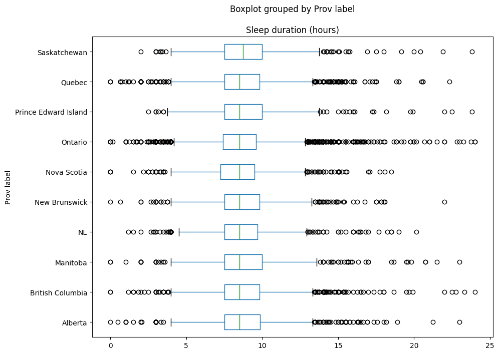
Boxplots are helpful for comparing the distributions between groups.

Sleephours_boxplot = prov_data_df.boxplot(
    column="Sleep duration (hours)", 
    by="Prov label", 
    figsize=(10,8),
    vert=False,
    # rot = 45, 
    grid=False
);

Sleephours_boxplot;

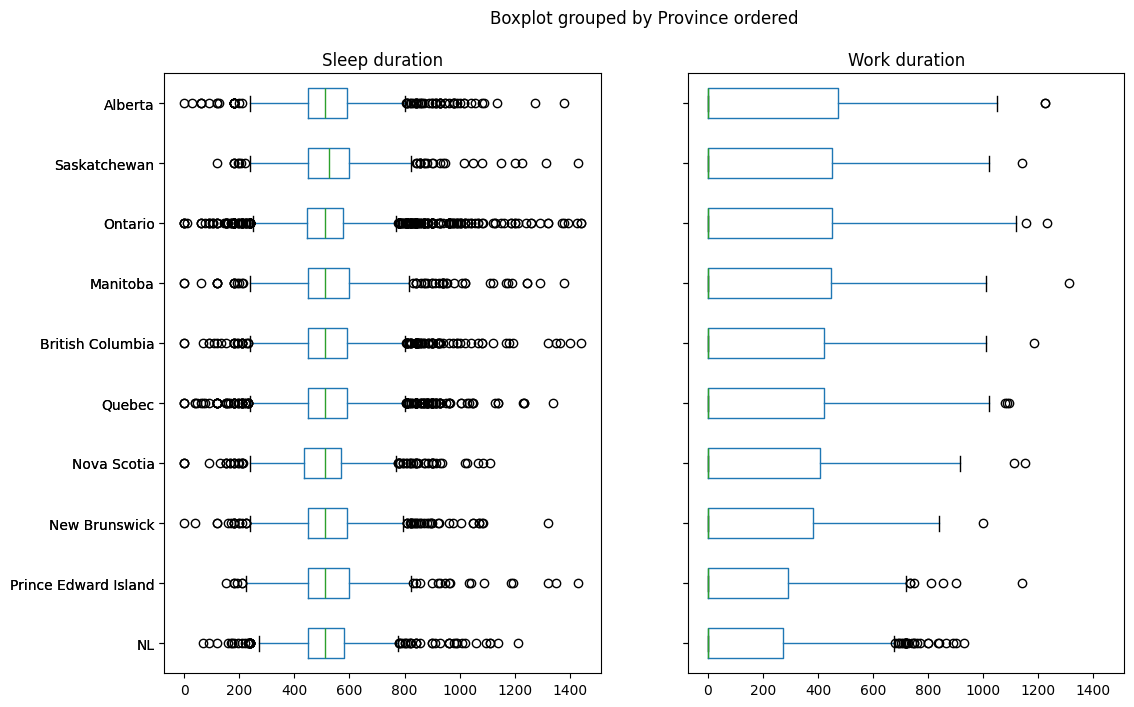
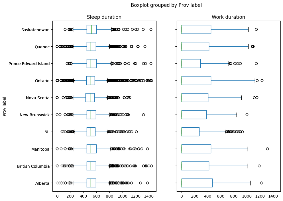
../../../_images/135928e1681f74a22eae33a68012a20620a067dc6867a4db57bf64d7b6b3d8f9.png

Compare the distribution of Sleep duration and Work duration by specifying the column parameter of DataFrame.boxplot as a list.

Sleepwork_boxplot = prov_data_df.boxplot(
    column = ["Sleep duration", "Work duration"], 
    by = "Prov label", 
    figsize = (10,8), 
    # rot = 90, 
    vert=False,
    grid = False, 
    layout = (1,2)
);

Sleepwork_boxplot;

../../../_images/fbc4254330d0b6f14b6bd46202a0b47e1062458a233e9206585cf30f813f2e2b.png

To further customize the look of your plots, see the documentation.

restwork_by_prov_mean.sort_values("Work duration")

	Sleep duration	Work duration	Total1	Total2
Prov label
NL	519.104339	133.946281	653.050620	653.050620
Prince Edward Island	534.065385	134.126923	668.192308	668.192308
New Brunswick	523.340265	148.428166	671.768431	671.768431
Nova Scotia	510.055019	158.398649	668.453668	668.453668
Quebec	525.554724	159.450461	685.005184	685.005184
British Columbia	528.488161	165.233753	693.721914	693.721914
Manitoba	529.791411	175.156442	704.947853	704.947853
Ontario	516.742869	177.705566	694.448434	694.448434
Saskatchewan	529.470905	182.572198	712.043103	712.043103
Alberta	522.629888	199.491620	722.121508	722.121508

prov_data_df["Province ordered"] = pd.Categorical(
    prov_data_df["Prov label"], 
    categories=restwork_by_prov_mean.sort_values("Work duration").index,
    ordered = True
)
Sleepwork_boxplot = prov_data_df.boxplot(
    column = ["Sleep duration", "Work duration"], 
    by = "Province ordered", 
    figsize = (12,8), 
    rot = 0, 
    grid = False, 
    layout = (1,2),
    vert = False
);
print(type(Sleepwork_boxplot[0]));
Sleepwork_boxplot[0].set_ylabel(None);
Sleepwork_boxplot;

<class 'matplotlib.axes._axes.Axes'>

../../../_images/3366b0eb310ba817465788ea973237526ef92871fa9c6bdcf0b27096a36925c7.png

Class 5: Data Transformations, Grouped Data, and Data Visualization

Contents

Class 5: Data Transformations, Grouped Data, and Data Visualization#

Last class#

This class#

Midterm Information#

Data Transformations#

Time use survey#

Subset the data#

Rename columns so that they are meaningful#

Create a new column in a pandas DataFrame#

What happened?#

Transform a column using if-then#

What happened?#

To create a new column in a pandas DataFrame using if-then/if-then-else logic#

Merging pandas DataFrames#

Is time spent resting different by province?#

Grouped summaries of data#

DataFrame Index#

Summing across rows of a DataFrame#

Two different ways to calulate row totals#

Statistical Variables#

Categorical variable

Nominal variable

Ordinal variable

Quantitative variable

Interval variable

Ratio variable

What’s the difference between a Statistical Variable and a Variable in python?#

Examples of implementing statistical variables in python#

Statistical Distributions#

What is the distribution of kids under 14 in Ontario?#

A bar plot of the distribution of kids under 14 in Ontario#

Summarizing the distribution of a quantitative variable#

Quantiles#

Variation#

Question#

Histograms#

Boxplots#

Anatomy of a Boxplot#