GGR274 Lab 5: Data Transformations, Grouped Data, and Data Visualization

Logistics

Like last week, our lab grade will be based on attendance and submission of a few small tasks to MarkUs during the lab session (or by 23:59 on Thursday).

Complete the tasks in this Jupyter notebook and submit your completed file to MarkUs. Here are the instructions for submitting to MarkUs (same as last week):

1. Download this file (Lab_5.ipynb) from JupyterHub. (See our JupyterHub Guide for detailed instructions.)

2. Submit this file to MarkUs under the lab5 assignment. (See our MarkUs Guide for detailed instructions.)

Note: Use autotests with this week”s lab to see if you are on the right track. It’s important to follow the steps so your answers match the solution in not only the way they appear on screen, but also in data types, in white spaces, in rounding, etc.

Lab 5 Introduction

In this lab, you will work with a data set called time_use_prov. This is a data set derived from the Statistics Canada General Social Survey’s (GSS) Time Use (TU) Survey Main File, as well as a data set containing information on aggregated provincial data. This week you will plot box plots, bar graphs, and use the logical operators from Week 4 material to develop subsets to visualize data on.

As usual, these labs are meant to facilitate your understanding of the material from lectures in a low-stakes environment. Please feel free to refer to your lecture content, collaborate with your peers, and seek out help from your TAs.

Task 1

Read CSV file "time_use_prov.csv" into a pandas DataFrame named prov_data.

import pandas as pd

prov_data = pd.read_csv("time_use_prov.csv")

prov_data.head()

/var/folders/0j/ybsv4ncn5w50v40vdh5jjlww0000gn/T/ipykernel_82472/3392639886.py:1: DeprecationWarning: 
Pyarrow will become a required dependency of pandas in the next major release of pandas (pandas 3.0),
(to allow more performant data types, such as the Arrow string type, and better interoperability with other libraries)
but was not found to be installed on your system.
If this would cause problems for you,
please provide us feedback at https://github.com/pandas-dev/pandas/issues/54466
        
  import pandas as pd

	Unnamed: 0	Participant ID	Urban/Rural	Age Group	Marital Status	sex	Kids under 14	Feeling Rushed	Sleep duration	Work duration	Prov_ab	Employment Rate	Pct house over 30	region	Income
0	0	10000	1	5	5	1	0	1	510	0	MB	61.7	11.4	Prairies	68147.0
1	1	10009	1	6	3	1	0	6	540	0	MB	61.7	11.4	Prairies	68147.0
2	2	10016	2	7	1	1	0	6	660	0	MB	61.7	11.4	Prairies	68147.0
3	3	10023	1	6	1	2	0	3	330	0	MB	61.7	11.4	Prairies	68147.0
4	4	10047	2	7	1	1	0	3	510	0	MB	61.7	11.4	Prairies	68147.0

Task 2

a) Create a new column in prov_data named "age_bin". The values of "age_bin" should be obtained from the "age" column in prov_data which has the values:

            Age group of respondent (groups of 10)

           VALUE  LABEL
               1  15 to 24 years
               2  25 to 34 years
               3  35 to 44 years
               4  45 to 54 years
               5  55 to 64 years
               6  65 to 74 years
               7  75 years and over
              96  Valid skip
              97  Don't know
              98  Refusal
              99  Not stated

"age_bin" should have the values "youth", "young", "middle", "senior" defined as :

• "youth" : ages 15-24

• "young" : ages 25-44

• "middle" : ages 45-64

• "senior" : ages 65+

# Solution

age = prov_data["Age Group"]

youth = (age == 1)
young = (age == 2) | (age == 3)
middle = (age == 4) | (age == 5)
senior = (age == 6) | (age == 7)

prov_data.loc[youth, "age_bin"] = "youth"
prov_data.loc[young, "age_bin"] = "young"
prov_data.loc[middle, "age_bin"] = "middle"
prov_data.loc[senior, "age_bin"] = "senior"

b) Compute the distribution of age_bin as counts, and store the count distribution in age_bin_count_dist. Then compute age_bin as a proportion of the total population, and store this in age_bin_prop_dist.

age_bin_count_dist = prov_data["age_bin"].value_counts()

age_bin_count_dist

age_bin
middle    6530
senior    4833
young     4724
youth     1303
Name: count, dtype: int64

age_bin_prop_dist = age_bin_count_dist / age_bin_count_dist.sum()

age_bin_prop_dist

age_bin
middle    0.375503
senior    0.277918
young     0.271650
youth     0.074928
Name: count, dtype: float64

c) Sort the values of age_bin_prop_dist in ascending order (smallest to largest) using the sort_values method. The code is

age_bin_prop_dist.sort_values(ascending=True, inplace=True)

(Not graded) The inplace=True parameter in sort_values modifies age_bin_prop_dist. What do you predict would happen to age_bin_prop_dist if we used age_bin_prop_dist.sort_values(ascending=True, inplace=False) instead?

age_bin_prop_dist.sort_values(ascending = True, inplace = True)

age_bin_prop_dist

age_bin
youth     0.074928
young     0.271650
senior    0.277918
middle    0.375503
Name: count, dtype: float64

age_bin_prop_dist.sort_values(ascending=True, inplace=False) will return a pd.Series with the values sorted. However, unlike using inplace=True, it will not update the values stored in age_bin_prop_dist.

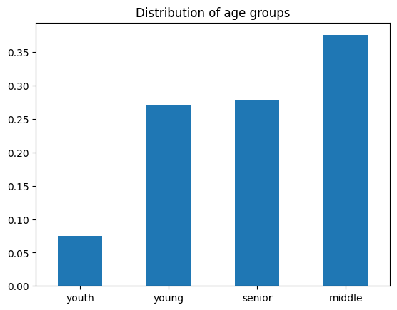
d) (Not graded) Create a bar plot of age_bin_prop_dist.

Feel free to explore different aesthetic options by changing paramters for the plotting function. (See the documentation here.)

age_bin_prop_dist.plot.bar()
age_bin_prop_dist.plot.bar(
    rot=0, 
    title="Distribution of age groups", 
    xlabel=""
)

<Axes: title={'center': 'Distribution of age groups'}>

Task 3

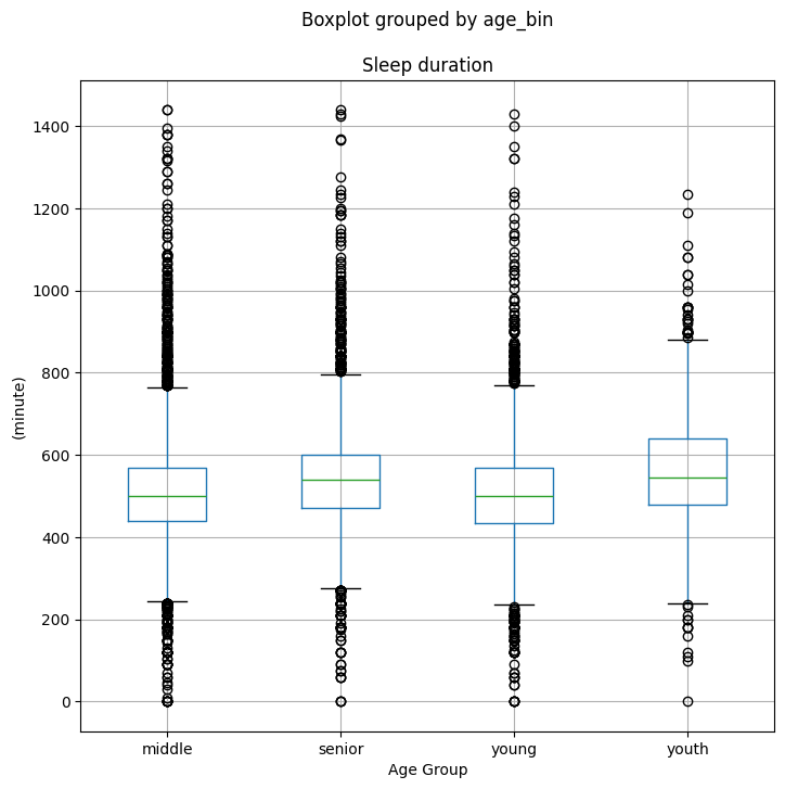
a) Create and store a boxplot of Sleep duration by age_bin to sleep_by_age_boxplots by completing the code below.

1. Use figsize=(8, 8) inside the pandas.DataFrame.boxplot() function;

2. Set the label on the x-axis to Age Group by using the .set_xlabel() method, as follows:

sleep_by_age_boxplots.set_xlabel("Age Group")

3. Set the label on the y-axis to (minute) by usign the .set_ylabel() method, as follows:

sleep_by_age_boxplots.set_ylabel("(minute)")

sleep_by_age_boxplots = prov_data.boxplot(
    column="Sleep duration", 
    by="age_bin", 
    figsize=(8,8)
);

sleep_by_age_boxplots.set_xlabel("Age Group");
sleep_by_age_boxplots.set_ylabel("(minute)");

# in case you don't see the plot without an error, try running the code below.
# sleep_by_age_boxplots.figure 

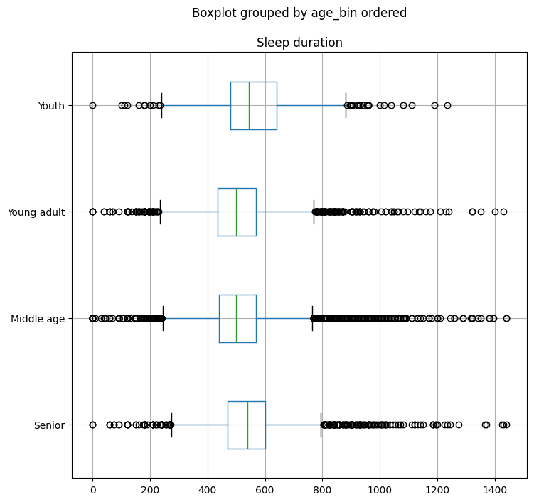
b) (Not graded) Feel free to customize a copy of the plot, sleep_by_age_boxplots_copy, further to your liking with the help of the documention.

Further customization. See documentation on pandas.Categorical for more information on the method.

sleep_by_age_boxplots_copy = sleep_by_age_boxplots

prov_data["age_bin ordered"] = pd.Categorical(
    prov_data["age_bin"],
    categories = [
        "senior",
        "middle",
        "young",
        "youth"
    ],
    ordered = True
)

sleep_by_age_boxplots_copy = prov_data.boxplot(
    column = "Sleep duration", 
    by = "age_bin ordered", 
    figsize = (8,8),
    vert = False
);

sleep_by_age_boxplots_copy.set_xlabel("");
sleep_by_age_boxplots_copy.set_ylabel("");
sleep_by_age_boxplots_copy.set_yticklabels([
    "Senior",
    "Middle age",
    "Young adult",
    "Youth"
]);

# in case you don't see the plot without an error, try running the code below.
# sleep_by_age_boxplots_copy.figure

sleep_by_age_boxplots.figure