GG274 Homework 11: Making a Map with GeoPandas

Logistics

Due date: The homework is due 23:59 on Tuesday, April 1.

You will submit your work on MarkUs. To submit your work:

1. Download this file (Homework_11.ipynb) from JupyterHub. (See our JupyterHub Guide for detailed instructions.)

2. Submit this file to MarkUs under the hw11 assignment. (See our MarkUs Guide for detailed instructions.) All homeworks will take place in a Jupyter notebook (like this one). When you are done, you will download this notebook and submit it to MarkUs.

Introduction

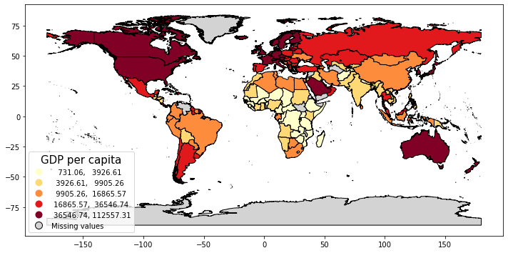
In this homework you will create a map of 2020 GDP (per capita, PPP in constant 2017 dollars) in each country around the world. First you’ll need to clean up the GDP data which has GDP values for multiple years. Then you’ll need to create a map of 2020 GDP classifying the data using 5 quantiles (e.g., quintiles).

import pandas as pd
import geopandas as gpd
import matplotlib.pyplot as plt
import mapclassify
import xlrd

Step 1 - Read the GDP data into a pandas DataFrame

a) The data is stored in gdp-per-capita-worldbank.csv .

Use the pandas function read_csv to read the data into a pandas DataFrame named gdp_data_df.

# Write your code below

gdp_data_df = pd.read_csv('gdp-per-capita-worldbank.csv')

b) Create a boolean Series called gdp_2020 that is True for the rows that represent GDP per capita in 2020, and False otherwise.

gdp_2020 = gdp_data_df['Year'] == 2020

c) Use gdp_data_df to create another DataFrame called gdp_2020_df that has three columns: 'Entity', 'Code', and 'GDP per capita' (in that order) and only has rows containing GDP data from 2020.

# Write your code below
important_cols = ['Entity', 'Code', 'GDP per capita']
gdp_2020_df = gdp_data_df.copy()

gdp_2020_df = gdp_2020_df[gdp_2020]
gdp_2020_df = gdp_2020_df[important_cols]

Step 2 - Bring in the world countries spatial data using geopandas as a GeoDataFrame.

a) Import the countries.geojson file using geopandas GeoDataFrame.from_file function and name the new GeoDataFrame as countries_gdf.

# Write your code below
countries_gdf = gpd.GeoDataFrame.from_file('countries.geojson')

Modify countries_gdf by renaming column ADMIN to Entity and column ISO_A3 to Code using a dictionary. Do this “in place” so that the original GeoDataFrame is modified, instead of creating a new GeoDataFrame.

# important_cols = countries_gdf.columns[[0,1,2]]
# colnames = {important_cols[0]: 'Entity',
#            important_cols[1]: 'Code',
#            important_cols[2]: 'geometry'}
colnames = {
    'ADMIN': 'Entity',
    'ISO_A3': 'Code'
}
countries_gdf.rename(columns=colnames, inplace=True)

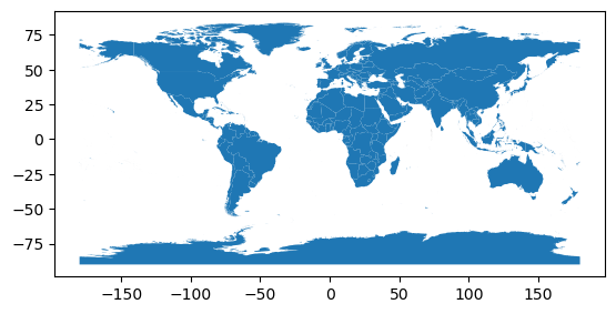
b) Create a basic figure of the new GeoDataFrame as a map using the plot function. Save the plot to a variable called countries_gdf_plot.

# Write your code below
countries_gdf_plot = countries_gdf.plot()

Step 3 - Join the spatial data with the GDP data

a) In this step you will merge the GDP data with the spatial countries data.

Use the merge function to do a left join (i.e., how='left') of the 2020 GDP DataFrame with the countries GeoDataFrame, using the column Code for the on argument.

Name the joined data countries_gdp_gdf.

# Write your code below

countries_gdp_gdf = countries_gdf.merge(gdp_2020_df, on='Code', how='left')

b) Why are we using a left join? Consider Aruba as an example. Hint: are the data consistently complete for all countries?

You may want to refer to the document of the merge function.

Write your answer in this cell.

Answer: not all countries have GDP reported for 2020. Countries like Aruba have GDP data for most years, but not 2020. The left join allows us to keep countries in the map, but that don’t have data.

Step 4 - Create a map that displays the 2020 GDP of world countries

In the below cell, create a map that displays GDP per capita in 5 quantiles. In the plot function use cmap = 'YlOrRd', edgecolor='black', ax=axes, scheme = 'quantiles', k = 5, and legend=True.

In addition, add the following two dictionaries in the plot function’s arguments:

missing_kwds={         'color': 'lightgrey',         'edgecolor': 'black',         'label': 'Missing values'}

legend_kwds={         'loc': 3,          'title': 'GDP per capita',         'title_fontsize': 23,         'fontsize': 15}

Save the map to countries_gdp_gdf_plot.

# Leave this code here: generate our figure/axes and set fig size
fig, axes = plt.subplots(1, 1, figsize = (12,12))

# Write your code below

countries_gdp_gdf_plot = countries_gdp_gdf.plot(
    column='GDP per capita',
    scheme='quantiles',
    k=5,
    cmap='YlOrRd', edgecolor='black', ax=axes, legend=True,
    missing_kwds={
        'color': 'lightgrey',
        'edgecolor': 'black',
        'label': 'Missing values'},
    legend_kwds={
        'loc': 3, 
        'title': 'GDP per capita',
        'title_fontsize': 15,
        'fontsize': 10
    }
)

Step 5 - Why do we use the missing kwds dictionary?

After looking at the code, write a sentence or two that interprets why we included missing_kwds in our plot function. Try rerunning the above code without the dictionary to better understand what it does.

Write your answer in this cell.

Answer: We use that code because it allows us to display the geometries of countries and regions that do not have 2020 GDP data.