Class 10

Mar. 19, 2024

By the end of this class, you’ll be able to:

• Fit linear regression;

• Know what is spatial data;

• Learn a new package geopandas;

• Do some basic spatial analysis (we’ll learn more in next 2 weeks!)

Review of linear regression

What is the effect of recent immigration on asthma rates in Toronto neighbourhoods?

Data

• Data from http://torontohealthprofiles.ca contains data on asthma and immigration for each neighbourhood in Toronto.

Sociodemographic data

• Read sociodemographic data from the excel file 1_socdem_neighb_2006-2.xls with sheet name socdem_2006 into pandas using read_excel.

import pandas as pd
import matplotlib.pyplot as plt 
import numpy as np
import seaborn as sns
from statsmodels.formula.api import ols

fname = '1_socdem_neighb_2006-2.xls'
sname = 'socdem_2006'
socdem_neighb = pd.read_excel(fname, sheet_name = sname, header = 10) # the table starts in row #11
socdem_neighb.head()

	Neighbourhood id	Neighbourhood Name	Total Population	% 19 and under	% 65 and over	% Living alone	% Aged 65+ living alone	% Lone parent families §	% 1 year mobility in population	Median household income before-tax $	...	% Less than high school education **	% With a University degree **	% No knowledge of English/French	% Recent immigrants-within 5 years	% Recent immigrants-within 10 years	% Immigrants	% Visible minority	Top 3 Home Languages for non-English speaking households, #1	Top 3 Home Languages for non-English speaking households, #2	Top 3 Home Languages for non-English speaking households, #3
0	1	West Humber-Clairville	32252	26.8	11.3	3.7	11.7	26.3	11.6	63413	...	18.4	22.9	5.4	12.2	22.1	60.0	77.9	Panjabi (Punjabi)	Gujarati	Spanish
1	2	Mount Olive-Silverstone-Jamestown	32127	32.2	8.1	4.1	15.4	31.5	15.7	48146	...	20.1	23.6	7.6	22.2	35.1	67.1	85.3	Panjabi (Punjabi)	Gujarati	Arabic
2	3	Thistletown-Beaumond Heights	9928	25.3	16.7	5.4	17.5	30.1	10.9	55032	...	16.7	20.7	5.0	9.7	19.3	55.9	53.8	Panjabi (Punjabi)	Italian	Spanish
3	4	Rexdale-Kipling	10725	23.6	18.3	10.2	28.8	33.3	13.2	52428	...	15.3	18.8	3.0	8.3	14.0	47.2	41.8	Spanish	Panjabi (Punjabi)	Croatian
4	5	Elms-Old Rexdale	9437	29.9	10.5	5.8	13.0	39.1	9.7	53779	...	15.2	18.8	3.6	9.8	18.2	53.8	60.5	Spanish	Italian	Urdu

5 rows × 28 columns

Which column should we select to measure immigration? There are several choices.

socdem_neighb.columns

Index(['Neighbourhood id', 'Neighbourhood Name', 'Total Population',
       '% 19 and under', '% 65 and over', '% Living alone',
       '% Aged 65+ living alone', '% Lone parent families §',
       '% 1 year mobility in population',
       'Median household income before-tax $',
       'Median household income after-tax $ ‡',
       '% Families-Incidence of low income before-tax',
       '% Families-Incidence of low income after-tax ‡',
       '% Individuals-Incidence of low income before-tax',
       '% Individuals-Incidence of low income after-tax ‡',
       '% Rented Dwellings', '% Unemployment rate *',
       '% Not in labour force *', '% Less than high school education **',
       '% With a University degree **', '% No knowledge of English/French',
       '% Recent immigrants-within 5 years',
       '% Recent immigrants-within 10 years', '% Immigrants',
       '% Visible minority',
       'Top 3 Home Languages for non-English speaking households, #1',
       'Top 3 Home Languages for non-English speaking households, #2',
       'Top 3 Home Languages for non-English speaking households, #3'],
      dtype='object')

• Let’s use '% Recent immigrants-within 5 years' to represent recent immigrants in a neighborhood.

• Later on we will want a few more sociodemographic columns, so let’s create a new DataFrame and rename the columns.

cols = ['Neighbourhood id', 'Neighbourhood Name', 
        'Median household income after-tax $ ‡', 
        '% Rented Dwellings', '% Unemployment rate *', 
        '% Recent immigrants-within 5 years', '% Visible minority']

socdem_neighb = socdem_neighb[cols]

colnames = {cols[0] : 'Neighbid',
            cols[1] : 'name',
            cols[2] : 'median_income',
            cols[3] : 'rented_dwell',
            cols[4] : 'unemployment',
            cols[5] : 'immigration5',
            cols[6] : 'vismin'}

socdem_neighb = socdem_neighb.copy()

socdem_neighb.rename(columns = colnames, inplace = True)

socdem_neighb.head()

	Neighbid	name	median_income	rented_dwell	unemployment	immigration5	vismin
0	1	West Humber-Clairville	56220	27.4	7.0	12.2	77.9
1	2	Mount Olive-Silverstone-Jamestown	43975	52.0	9.9	22.2	85.3
2	3	Thistletown-Beaumond Heights	49800	34.4	6.3	9.7	53.8
3	4	Rexdale-Kipling	46033	45.1	7.7	8.3	41.8
4	5	Elms-Old Rexdale	48055	41.2	7.8	9.8	60.5

Asthma data

• Read data from the excel file 1_ahd_neighb_db_ast_hbp_mhv_copd_2007.xls with sheet name 1_ahd_neighb_asthma_2007 into pandas using read_excel.

fname = '1_ahd_neighb_db_ast_hbp_mhv_copd_2007.xls'
sname = '1_ahd_neighb_asthma_2007'

asthma_neighb = pd.read_excel(fname, sheet_name = sname, header = 11) #the table starts with row #12
asthma_neighb.head()

	Unnamed: 0	Unnamed: 1	Demographics ª	% With asthma	LL (95% CI)	UL (95% CI)	Demographics ª.1	% With asthma.1	LL (95% CI) .1	UL (95% CI) .1	...	Demographics ª.7	% With asthma.7	LL (95% CI) .7	UL (95% CI) .7	Demographics ª.8	% With asthma.8	LL (95% CI) .8	UL (95% CI) .8	Rate Ratio**.2	H/L/NS.2
0	1	West Humber-Clairville	11977	9.7	9.2	10.2	11770	10.6	10.0	11.2	...	4435	12.3	11.3	13.3	8921	10.9	10.3	11.6	1.07	H
1	2	Mount Olive-Silverstone-Jamestown	11157	7.9	7.4	8.4	11462	10.2	9.6	10.8	...	3819	13.5	12.5	14.6	7726	11.2	10.5	11.9	1.10	H
2	3	Thistletown-Beaumond Heights	3307	9.4	8.4	10.4	3322	10.5	9.5	11.6	...	1307	12.3	10.5	14.1	2587	10.8	9.6	12.0	1.06	NS
3	4	Rexdale-Kipling	3317	9.7	8.7	10.7	3438	13.0	11.9	14.2	...	1468	13.2	11.5	14.9	2897	10.4	9.3	11.5	1.02	NS
4	5	Elms-Old Rexdale	3209	10.2	9.1	11.2	3379	13.0	11.8	14.1	...	1314	15.1	13.1	17.0	2610	11.8	10.6	13.0	1.16	H

5 rows × 44 columns

• The asthma rates are broken down by sex and age.

• Which rates should we choose?

• For this example, let’s select asthma rates for both sexes age 20 - 64.

asthma_neighb.columns

Index(['Unnamed: 0', 'Unnamed: 1', 'Demographics ª', '% With asthma',
       'LL (95% CI) ', 'UL (95% CI) ', 'Demographics ª.1', '% With asthma.1',
       'LL (95% CI) .1', 'UL (95% CI) .1', 'Demographics ª.2',
       '% With asthma.2', 'LL (95% CI) .2', 'UL (95% CI) .2', 'Rate Ratio**',
       'H/L/NS', 'Demographics ª.3', '% With asthma.3', 'LL (95% CI) .3',
       'UL (95% CI) .3', 'Demographics ª.4', '% With asthma.4',
       'LL (95% CI) .4', 'UL (95% CI) .4', 'Demographics ª.5',
       '% With asthma.5', 'LL (95% CI) .5', 'UL (95% CI) .5', 'Rate Ratio**.1',
       'H/L/NS.1', 'Demographics ª.6', '% With asthma.6', 'LL (95% CI) .6',
       'UL (95% CI) .6', 'Demographics ª.7', '% With asthma.7',
       'LL (95% CI) .7', 'UL (95% CI) .7', 'Demographics ª.8',
       '% With asthma.8', 'LL (95% CI) .8', 'UL (95% CI) .8', 'Rate Ratio**.2',
       'H/L/NS.2'],
      dtype='object')

# Select the neghborhood_id, neighborhood_name, and both sexes with asthma

important_cols = asthma_neighb.columns[[0, 1, 11]]

colnames = {important_cols[0]: 'Neighbid',
           important_cols[1] : 'name',
           important_cols[2] : 'asthma_pct'}

asthma_rates = asthma_neighb.copy()

asthma_rates = asthma_rates[important_cols]

asthma_rates.rename(columns = colnames, inplace=True)

asthma_rates.head()

	Neighbid	name	asthma_pct
0	1	West Humber-Clairville	10.2
1	2	Mount Olive-Silverstone-Jamestown	9.1
2	3	Thistletown-Beaumond Heights	10.0
3	4	Rexdale-Kipling	11.4
4	5	Elms-Old Rexdale	11.6

Merge Sociodemographic and asthma data

• To examine the relationship between asthma and immigration we will need to merge socdem_neighb and asthma_rates.

• The DataFrames can be merged on neighbourhood id.

# Two datasets are merged based on neighborhood id

asthma_socdem = asthma_rates.merge(socdem_neighb, left_on='Neighbid', right_on='Neighbid')

asthma_socdem.head()

	Neighbid	name_x	asthma_pct	name_y	median_income	rented_dwell	unemployment	immigration5	vismin
0	1	West Humber-Clairville	10.2	West Humber-Clairville	56220	27.4	7.0	12.2	77.9
1	2	Mount Olive-Silverstone-Jamestown	9.1	Mount Olive-Silverstone-Jamestown	43975	52.0	9.9	22.2	85.3
2	3	Thistletown-Beaumond Heights	10.0	Thistletown-Beaumond Heights	49800	34.4	6.3	9.7	53.8
3	4	Rexdale-Kipling	11.4	Rexdale-Kipling	46033	45.1	7.7	8.3	41.8
4	5	Elms-Old Rexdale	11.6	Elms-Old Rexdale	48055	41.2	7.8	9.8	60.5

A regression model of asthma on immigration

Plot the data

• What are the dependent and independent variables?

• Does the relationship look linear?

sns.regplot(y = 'asthma_pct', x = 'immigration5', data = asthma_socdem, ci = None);

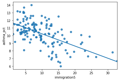
Describe the relationship between asthma and immigration.

Fit the regression model

reg_asthmaimm = ols('asthma_pct ~ immigration5', data = asthma_socdem) # setup the model

reg_asthmaimm_fit = reg_asthmaimm.fit() # estimate/fit the model 

Statistical summary of the regression model

reg_asthmaimm_summ = reg_asthmaimm_fit.summary()

reg_asthmaimm_summ.tables[1]

	coef	std err	t	P>|t|	[0.025	0.975]
Intercept	11.8266	0.218	54.328	0.000	11.396	12.257
immigration5	-0.1597	0.019	-8.475	0.000	-0.197	-0.122

The regression model is the equation:

\[\texttt{asthma_pct} = 11.8266 - 0.1597 \times \texttt{immigration5}\]

• The slope indicates that for a 1% increase in immigration in the past 5 years the percentage of asthma cases in a neighbourhood decrease by 0.1597%.

• The y-intercept indicates that when a neighbourhood has 0% immigration the past 5 years then asthma rates are 11%.

• Are there any neighbourhoods with 0% immigration in the past 5 years?

asthma_socdem['immigration5'].describe()

count    140.000000
mean       9.864286
std        6.037045
min        1.200000
25%        4.975000
50%        8.650000
75%       13.100000
max       32.800000
Name: immigration5, dtype: float64

• The y-intercept in regression models often doesn’t have a sensible interpretation, but is often mathematically important for regression to work well.

Accuracy of the regression model

reg_asthmaimm_fit.rsquared

0.34233239704200125

plt.scatter(x = reg_asthmaimm_fit.fittedvalues , y = reg_asthmaimm_fit.resid)
plt.axhline(y = 0)
plt.xlabel('fitted values')
plt.ylabel('residuals')

Text(0, 0.5, 'residuals')

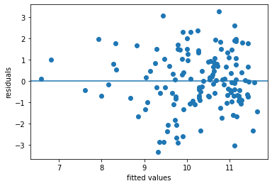
• The R-squared statistics indicates a relatively good explanation of the model (quite larger than 0)

• The residual plot indicates some important variables are missing, as we can see larger abolute values as fitted values increase (not a random distributed pattern)

Summary

Therefore, we can conclude that the immigration rate in recent 5 years in a neighborhood is negatively associated with the prevalence of asthma in the neighborhood.

Why not causal relationship?

What is the implication?

Training and testing a model

• Ideally we could assess the accuracy of this linear regression model on a new set of data (i.e., immigration rates in Toronto neighbourhoods in future years.)

• But, we don’t have this data.

• One trick that data scientists use to fit the model on part of the data (training data) and use the remaining part (testing data) to test the accuracy.

• If we only have one data set then the training data can be obtained by randomly selecting rows from the data to fit the regression model, then the remaining rows can be used to test the accuracy of the model.

Splitting a pandas DataFrame by index

data = {'a' : [1, 2, 3, 4, 5]}

df = pd.DataFrame(data)

df.index

RangeIndex(start=0, stop=5, step=1)

A Boolean array that is True if the index is 0 or 1 and False otherwise.

df.index.isin([0,1])

array([ True,  True, False, False, False])

df[df.index.isin([0,1])]

	a
0	1
1	2

To create a Boolean series that is False if the index is 0 or 1 and True otherwise we can negate df.index.isin([0,1]) this Boolean series using the ~ operator ~df.index.isin([0,1])

~df.index.isin([0,1])

array([False, False,  True,  True,  True])

df[~df.index.isin([0,1])]

	a
2	3
3	4
4	5

Creating training and test data sets from a single dataset

Step 1:

• split the data into a training set with 75% of the rows.

• use the remaining 25% of the data for testing.

np.random.seed(11) # for reproducibility

# randomly select 75% of neighbourhoods
reg_df_train = asthma_socdem.sample(frac = 0.75, replace = False) 

# get index of training data
train_index = reg_df_train.index

• Exclude indicies from reg_df_train using pandas isin function.

# exclude rows in training to define test data
reg_df_test = asthma_socdem[~asthma_socdem.index.isin(train_index)]

print(asthma_socdem.shape)

print(reg_df_train.shape)

print(reg_df_test.shape)

(140, 9)
(105, 9)
(35, 9)

Step 2: Fit the regression model on the training data

reg_train = ols('asthma_pct ~ immigration5', data = reg_df_train) # setup the model

reg_train_fit = reg_train.fit() # estimate/fit the model 

Step 3: Compute fitted values using training data

# use the model fit on the training data to predict asthma rates
# from the test set. 

predvalues_train = reg_train_fit.fittedvalues

# Another way to compute
# predvalues_train = reg_train_fit.predict(reg_df_train['immigration5'])

Step 4: Evaluate accuracy using root mean-squared error on training data

• Another measure of accuracy of regression models.

• Compares observed values of the dependent variable with the predicted values.

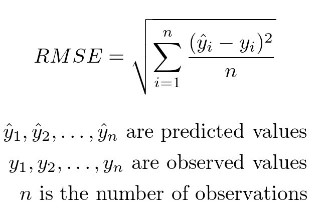
It can be computed using the rmse function from statsmodels.

# Compute root mean-squared error for the training data.
from statsmodels.tools.eval_measures import rmse

rmse(predvalues_train, reg_df_train['asthma_pct'])

1.3987103239995489

• The observed asthma rates deviate from the predicted asthma rates in each neighbourhood by 1.4% in the training set.

• Is this an acceptable prediction error?

• Let’s examine the accuracy of the linear regression model on the test set

Step 5: Evaluate the accuracy of regression model on the test data using root mean-squared error

• Compute predictions using test data

predvalues_test = reg_train_fit.predict(reg_df_test['immigration5'])

• Now compute the root mean-squared error for the test data using the model fit on the training data.

rmse(predvalues_test, reg_df_test['asthma_pct'])

1.1096219805062997

Conclusion of data analysis using linear regression model

• The regression model appears to provide an accurate fit the data, although both the scatter plot and plot of residuals indicate that there is a lot of variation in asthma rates in neighbourhoods when the immigrations rates are small (between 10%-20%).

• As the percentage of immigrants to a neighbourhood within the last 5 years increases, the asthma rates will decreases.

• Regression analyses on aggregated data such as neighbourhoods can be misleading when compared to non-aggregated data.

Are there other sociodemographic factors in our data that might effect asthma rates?

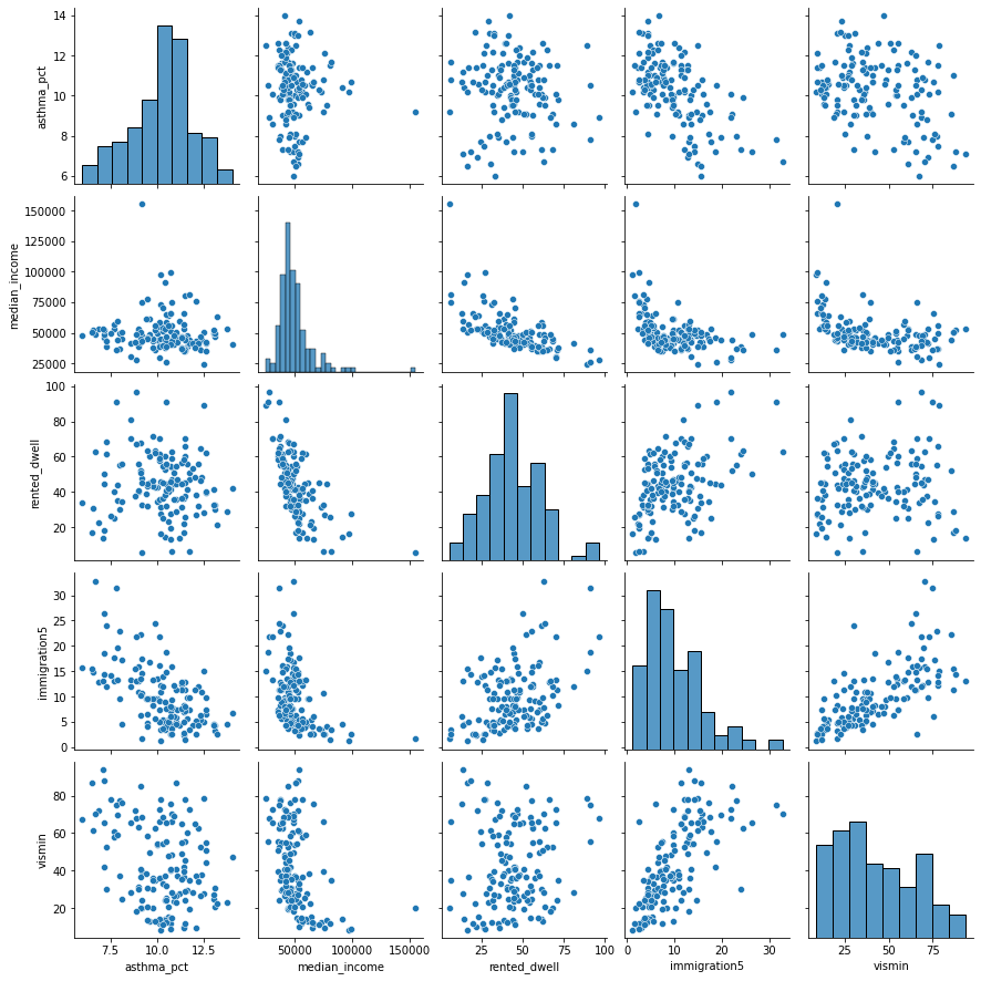
• Let’s create a matrix scatter plot using pairplot in the seaborn library.

• pairplot will visualize paired relationship between variables in a dataset.

asthma_socdem.columns

Index(['Neighbid', 'name_x', 'asthma_pct', 'name_y', 'median_income',
       'rented_dwell', 'unemployment', 'immigration5', 'vismin'],
      dtype='object')

# reduce the column for better presentation
to_show = ['asthma_pct','median_income','rented_dwell','immigration5','vismin']
sns.pairplot(asthma_socdem[to_show]);

• Let’s consider median income

• Fit the regression model on all the data and produce a statistical summary.

reg_asthmaimmunem = ols('asthma_pct ~ immigration5 + median_income', data = asthma_socdem) # setup the model

reg_asthmaimmunem_fit = reg_asthmaimmunem.fit() # estimate/fit the model 

reg_asthmaimmunem_summ = reg_asthmaimmunem_fit.summary()

reg_asthmaimmunem_summ.tables[1]

	coef	std err	t	P>|t|	[0.025	0.975]
Intercept	14.3041	0.497	28.758	0.000	13.321	15.288
immigration5	-0.2054	0.019	-10.750	0.000	-0.243	-0.168
median_income	-4.048e-05	7.45e-06	-5.431	0.000	-5.52e-05	-2.57e-05

• Notice that the slope estimate (coefficient) for median_income is 0, but so is the p-value and range of plausible values.

• That seems odd. What’s happening?

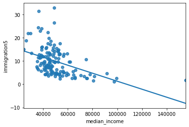
• We can see from the scatter plot that immigration5 and median_income have a linear relationship.

• When two variables have a linear relationship multiple linear regression models produce strange results.

• It’s important that independent variables in a multiple regression model are unrelated.

sns.regplot(y = 'immigration5', x = 'median_income', data = asthma_socdem, ci = None);

A quick review of linear regression

• Step 1: prepare data (Which dataset I want to import? Which variables I want to analyze? How I can ‘wrangle’ the data, i.e., produce new variables and merge them into one dataframe for further analysis?)

• Step 2: Explore pair relationship (Using sns.pairplot to explore potential relationships. Is there a linear relationship?)

• Step 3: Fit model

• Step 4: Accuracy (Which indicators I want to use? e.g., r-squared, residual plot, RMSE)

• Step 5: Display the full model and explain (What does the model mean?)

Introduction to spatial data

Why Spatial Data Matters

What are spatial data?

Spatial data are data that have some geographic attribute(s). So you can think of it like each row having a pointer to where the row goes on a map.

Why do we want spatial data?

By locating things on a map, we can look for how certain variables present vary across space. We can look for things like clustering of high values or cold spots (aka hot spots/cold spots) or dispersal. Patterns across space can reveal interesting drivers of social phenomena.

Types of Spatial Data

raster data & vector data

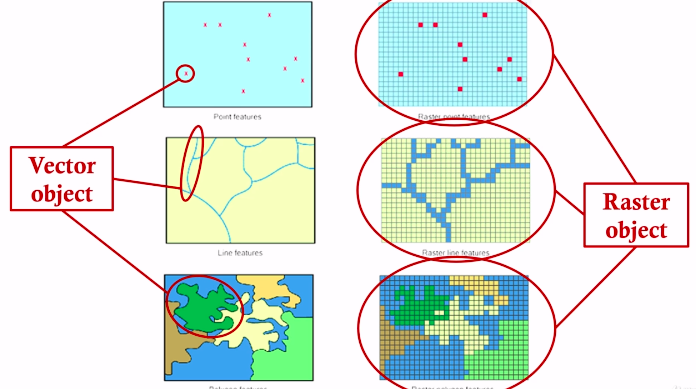
Raster data

For example, satellite and aerial images

Vector data

For example, points, lines, and polygons

How are these data stored in a computer?

There are many ways!

Generally raster data are stored as a matrix

Vector data is stored in many different ways…

Two common ones are geojson and shapefiles.

What are these files made of?

Geojson is pretty straightforward:

Shapefiles are more complicated and involve multiple distinct files that contain information about spatial locations, coordinate systems and projections, attributes, etc. We’ll focus on geojson for this class.

Introducing GeoPandas

How do we work with spatial data in python?

We’re going to use something called ‘geopandas’

https://geopandas.org/en/stable/

There are a few other libraries that we need, like mapclassify. There are a lot of different tools out there, but we’ll stick to these two (and the xls reader) for today

# # Let's install and then load libraries
# import sys
# !{sys.executable} -m pip install geopandas
# !{sys.executable} -m pip install mapclassify
# !{sys.executable} -m pip install xlrd

import pandas as pd
import geopandas as gpd
import matplotlib.pyplot as plt
import mapclassify
import xlrd

Now we want to import a spatial data file.

We’ll be working with two spatial data files today: Toronto_Neighbourhoods.geojson and toronto_rails.geojson

We’ll also use the health data we were playing with last week: 1_ahd_neighb_db_ast_hbp_mhv_copd_2007.xls

To load the spatial data we need to create something known as a geodataframe:

nbrhd = gpd.GeoDataFrame.from_file("Toronto_Neighbourhoods.geojson") ## Like pd.read_xxx(file_name)
nbrhd.head()

	AREA_ATTR_ID	AREA_DESC	AREA_ID	AREA_LONG_CODE	AREA_NAME	AREA_SHORT_CODE	CLASSIFICATION	CLASSIFICATION_CODE	LATITUDE	LONGITUDE	OBJECTID	PARENT_AREA_ID	Shape__Area	Shape__Length	X	Y	_id	geometry
0	26005521	Casa Loma (96)	2480141	096	Casa Loma (96)	096	None	None	None	None	17545105	None	3.678385e+06	8214.176485	None	None	1	POLYGON ((-79.41469 43.67391, -79.41485 43.674...
1	26005520	Annex (95)	2480140	095	Annex (95)	095	None	None	None	None	17545121	None	5.337192e+06	10513.883143	None	None	2	POLYGON ((-79.39414 43.66872, -79.39588 43.668...
2	26005519	Caledonia-Fairbank (109)	2480139	109	Caledonia-Fairbank (109)	109	None	None	None	None	17545137	None	2.955857e+06	6849.911724	None	None	3	POLYGON ((-79.46021 43.68156, -79.46044 43.681...
3	26005444	Woodbine Corridor (64)	2480064	064	Woodbine Corridor (64)	064	None	None	None	None	17545153	None	3.052518e+06	7512.966773	None	None	4	POLYGON ((-79.31485 43.66674, -79.31660 43.666...
4	26005443	Lawrence Park South (103)	2480063	103	Lawrence Park South (103)	103	None	None	None	None	17545169	None	6.211341e+06	13530.370002	None	None	5	POLYGON ((-79.41096 43.70408, -79.41165 43.703...

# Let's look at the geometry column - this is the data that 
# describes the polygon representing the first neighbourhood

print(nbrhd.loc[0,'geometry'])

POLYGON ((-79.41469317817781 43.6739104164259, -79.41484930122832 43.6743388247927, -79.4155279126094 43.67606998537741, -79.4157867581137 43.6767302521386, -79.4164385645546 43.6783329020511, -79.4165782543862 43.6787785512344, -79.4167583944682 43.6792484522149, -79.41698203537291 43.6798247440047, -79.4170902471251 43.6801047004014, -79.4174797570886 43.681051830379, -79.4176666295158 43.6815699096212, -79.4176976020857 43.68163169892501, -79.4178116560388 43.6819252777403, -79.4181213711598 43.6827105222857, -79.4182734938897 43.6830961662335, -79.418301440907 43.683167503583, -79.4184313411692 43.6834966841996, -79.4184870757371 43.6836294842548, -79.4185410795905 43.6837582054538, -79.4184092922561 43.683786393574, -79.4182955283344 43.6834937157887, -79.4154265333151 43.684065660547, -79.4135200432832 43.6844456915062, -79.4134087861596 43.6844695957643, -79.4134686959176 43.6846245536214, -79.4124643275333 43.6848288476745, -79.4118960009694 43.6849418545125, -79.4126020656339 43.6866857692443, -79.4128218223812 43.687229039671, -79.4122731860895 43.687340632143, -79.4123095851789 43.6874306640936, -79.4124449310775 43.6877690817767, -79.4125749764611 43.6881026705283, -79.4126022442033 43.68820308289101, -79.4126262355444 43.6883388768546, -79.412631283351 43.6884334123732, -79.4126432068819 43.6885168725437, -79.4126690850027 43.6886690142942, -79.4121798023448 43.6887725684515, -79.4121317450359 43.688782747996, -79.4094911620232 43.6893416576956, -79.4095159141932 43.6894373160946, -79.4079543147094 43.6897847976179, -79.4064026019847 43.6900806794424, -79.4048987011668 43.6903958607535, -79.4030176369546 43.6907821281771, -79.4030622386805 43.6907397518989, -79.403084589916 43.6906872662864, -79.4030847025454 43.6906327275232, -79.40233853963132 43.6887211977866, -79.4014954899744 43.6866406966408, -79.401126389152 43.6857160700657, -79.400841057476 43.6850272500519, -79.4005303647662 43.6843098010236, -79.4002092949982 43.6835267044631, -79.4001688947727 43.6834159800984, -79.3998035302044 43.6825434875815, -79.3992154226597 43.6811276314469, -79.3990654446524 43.6807665464922, -79.3989394746847 43.6804604265612, -79.3987331620365 43.679962228305, -79.3985629657772 43.6795542728627, -79.3983515160598 43.6790391648102, -79.3981409020124 43.6785307360415, -79.3980121612171 43.6782038734666, -79.3979440512351 43.6780262977103, -79.3979313672526 43.6779949618024, -79.397997906573 43.6779648847871, -79.39810766305662 43.6779154844303, -79.3982178162304 43.677866084320804, -79.3983283660932 43.677816684457504, -79.3984396598895 43.6777672941492, -79.3985509707706 43.677722377402, -79.39866305797811 43.6776729695768, -79.3987751498381 43.6776280623042, -79.39888799806091 43.677583155590305, -79.3990012429834 43.6775382491152, -79.399114879728 43.6774888512157, -79.3992025285702 43.6774574239244, -79.3992901799736 43.6774169952501, -79.3993786050701 43.6773810678483, -79.3994674269127 43.677345149728104, -79.3995566132194 43.6773137235166, -79.3996462037999 43.6772777969312, -79.3997357818565 43.6772418792657, -79.3998261336784 43.6772104448643, -79.3999168946437 43.6771790287522, -79.4000076183382 43.6771475945326, -79.4000991356532 43.6771161699357, -79.4001906603179 43.6770802536138, -79.4002825618979 43.6770488292052, -79.4003752372778 43.6770218970549, -79.40046791256 43.6769949738305, -79.4005609796537 43.6769635502124, -79.4006540144064 43.6769366361508, -79.40074786265342 43.6769052040578, -79.4008416959652 43.6768827821947, -79.4009359160751 43.6768513592708, -79.4010305181557 43.6768289379187, -79.4011394914127 43.6767930269395, -79.40124844475712 43.6767616164984, -79.4013577948506 43.6767302062957, -79.4014675168886 43.6766987963088, -79.401577635645 43.6766674045606, -79.4016877469976 43.6766404773541, -79.4017982426678 43.6766135773755, -79.401909142447 43.6765821679758, -79.4020200223858 43.6765552591109, -79.4021313064015 43.6765238498247, -79.4022429725496 43.6765014420761, -79.4023546335109 43.6764745335542, -79.4024666788314 43.6764476252511, -79.4025787240519 43.6764207168379, -79.4026915556349 43.6763983006426, -79.40280397272 43.67637139232491, -79.402883149386 43.6763541860873, -79.4029167917251 43.6763489758964, -79.4030299826882 43.6763265686732, -79.4031435776805 43.6762996520191, -79.4049670168388 43.6759208047062, -79.4073338149418 43.675429007407, -79.407847991862 43.67532218132661, -79.4113608949251 43.6745959152122, -79.4121860970333 43.6744315128604, -79.4137161812489 43.6741115018232, -79.4146748682077 43.6739143093347, -79.41469317817781 43.6739104164259))

# Otherwise we can continue to treat the variable like a dataframe ... 
# it's what we have been doing all along!

nbrhd_names = nbrhd["AREA_NAME"]
type(nbrhd_names)

pandas.core.series.Series

Now if we want to make a map, what do we do?

It’s easy! You can “plot” a geodataframe and geopandas will make it a map!

nbrhd.plot() 

<AxesSubplot:>

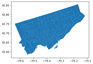
That’s nice…

But we want to be a little more sophisticated with our maps.

The next cell goes through a better way to create a map “figure”.

Let’s first create Figure and Axes objects.

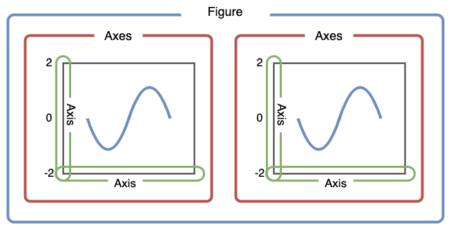
First, let’s use plt.subplots to create a figure variable “fig” and an axes variables called “ax”.

The first line of code sets the stage - it says how many images - by rows/columns, and we can set other figure attributes in here, like figure size using figsize.

To plot the map, we need to call the plot command .plot like before, but this time we want to say which ‘cell’ or ax cell it will go in, i.e., ax=axes. We also can use the column parameter to shade each row (that represents a polygon) by an attribute value.

fig, axes = plt.subplots(1, 1, figsize = (12,12))

print(type(fig)) #Figure object is like the sheet we are drawing on
print(type(axes))  #AxesSubplots are like cells within the sheet

nbrhd.plot(column = "AREA_NAME", ax = axes);

<class 'matplotlib.figure.Figure'>
<class 'matplotlib.axes._subplots.AxesSubplot'>

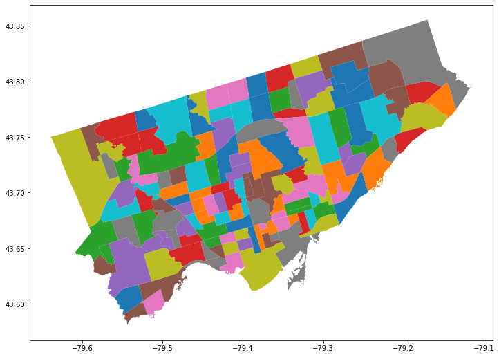
What if we want to do 2 maps in one figure?

fig, axes = plt.subplots(1, 2)

#notice there are just 2 things in the axes object
print(axes.shape)

# pick the first cell in the figure
ax = axes[0]
nbrhd.plot(column = "AREA_NAME",
           ax=ax)

# pick the second cell in the figure
ax = axes[1]
nbrhd.plot(ax=ax)

#resize
current_fig = plt.gcf() #get current figure aka gcf
current_fig.set_size_inches(15,10) #set figure width
current_fig.savefig('torontomaps.png',dpi=100) #export maps as an image file!

(2,)

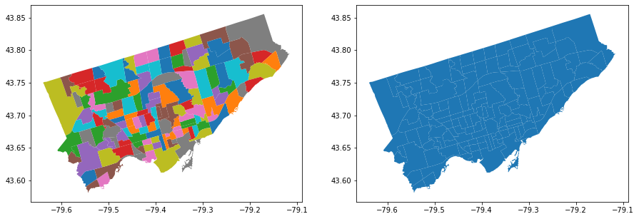
A note about axes:

• if you only has one ‘axes’ (i.e., plt.subplots(1,1)) then you can just say ax = axes

• if you have a 1 row and multiple columns or multiple rows and 1 column, then you would say ax = axes[n] where n is the axes cell you’d like to put the figure in

• if you have a matrix of cells of axes (i.e., plt.subplots(2,2)) then you need to say ax = axes[n][m] where n is the row number and m is the column number of the cell

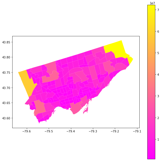
Let’s try with a column that contains a number… what happens there?

let’s also add a new parameter “cmap” = color map and a legend.

This link will provide more info on other things we can do with plotting geodataframes: https://geopandas.org/en/stable/docs/reference/api/geopandas.GeoDataFrame.plot.html

fig, axes = plt.subplots(1,1)

# We want to plot the area of each neighborhood
nbrhd.plot(column = "Shape__Area", ax = axes, 
           cmap = "spring", legend = True)

current_fig = plt.gcf()
current_fig.set_size_inches(10, 10)

let’s try again with neighbourhoods:

#another way to resize
fig, axes = plt.subplots(1,1, figsize = (15,15))


nbrhd.plot(column = "AREA_NAME", ax = axes,
           cmap = "Pastel1", legend = True)

<AxesSubplot:>

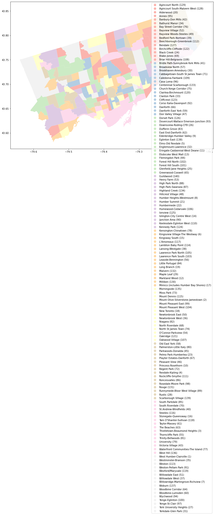
… These are silly maps. Who cares how big the neighbourhoods are or who can deal with a weird pastel map with a legend that is way too big…

We want to know what is happening inside of them!

How do we bring two pieces of info together? How do we bring data from a table into a geodataframe?

We can use joins! Remember those?

How do we bring data from a table into a geodataframe?

We can use merge, just like what we did before!

Let’s join the asthma rates into the neighborhood and map them out.

# simplify the geodataframe ready

important_spat_cols = nbrhd.columns[[4, 5, 17]]
colnames_spat = {important_spat_cols[0]: 'name',
           important_spat_cols[1] : 'nbrhd_spat_id',
           important_spat_cols[2] : 'geometry'}

nbrhd_simple = nbrhd.copy()

nbrhd_simple = nbrhd_simple[important_spat_cols]

nbrhd_simple.rename(columns = colnames_spat, inplace=True)

# Notice that the "nbrhd_spat_id" is a string and not a number... that may be an issue
print("The data type of nbrhd_spat_id is: ", type(nbrhd_simple["nbrhd_spat_id"][0]))
nbrhd_simple.head()

The data type of nbrhd_spat_id is:  <class 'str'>

	name	nbrhd_spat_id	geometry
0	Casa Loma (96)	096	POLYGON ((-79.41469 43.67391, -79.41485 43.674...
1	Annex (95)	095	POLYGON ((-79.39414 43.66872, -79.39588 43.668...
2	Caledonia-Fairbank (109)	109	POLYGON ((-79.46021 43.68156, -79.46044 43.681...
3	Woodbine Corridor (64)	064	POLYGON ((-79.31485 43.66674, -79.31660 43.666...
4	Lawrence Park South (103)	103	POLYGON ((-79.41096 43.70408, -79.41165 43.703...

#get the asthma data

fname = '1_ahd_neighb_db_ast_hbp_mhv_copd_2007.xls' #file name
sname = '1_ahd_neighb_asthma_2007' #sheet name in excel file

#store excel sheet with asthma data in a dataframe variable
asthma_neighb = pd.read_excel(fname, sheet_name = sname, header = 11)
asthma_neighb.head()

	Unnamed: 0	Unnamed: 1	Demographics ª	% With asthma	LL (95% CI)	UL (95% CI)	Demographics ª.1	% With asthma.1	LL (95% CI) .1	UL (95% CI) .1	...	Demographics ª.7	% With asthma.7	LL (95% CI) .7	UL (95% CI) .7	Demographics ª.8	% With asthma.8	LL (95% CI) .8	UL (95% CI) .8	Rate Ratio**.2	H/L/NS.2
0	1	West Humber-Clairville	11977	9.7	9.2	10.2	11770	10.6	10.0	11.2	...	4435	12.3	11.3	13.3	8921	10.9	10.3	11.6	1.07	H
1	2	Mount Olive-Silverstone-Jamestown	11157	7.9	7.4	8.4	11462	10.2	9.6	10.8	...	3819	13.5	12.5	14.6	7726	11.2	10.5	11.9	1.10	H
2	3	Thistletown-Beaumond Heights	3307	9.4	8.4	10.4	3322	10.5	9.5	11.6	...	1307	12.3	10.5	14.1	2587	10.8	9.6	12.0	1.06	NS
3	4	Rexdale-Kipling	3317	9.7	8.7	10.7	3438	13.0	11.9	14.2	...	1468	13.2	11.5	14.9	2897	10.4	9.3	11.5	1.02	NS
4	5	Elms-Old Rexdale	3209	10.2	9.1	11.2	3379	13.0	11.8	14.1	...	1314	15.1	13.1	17.0	2610	11.8	10.6	13.0	1.16	H

5 rows × 44 columns

#let's simplify this by only pulling a few relevant columns
important_cols = asthma_neighb.columns[[0, 1, 11]]
colnames = {important_cols[0]: 'Neighbid',
           important_cols[1] : 'name',
           important_cols[2] : 'asthma_pct'}

asthma_rates = asthma_neighb.copy()

asthma_rates = asthma_rates[important_cols]

asthma_rates.rename(columns = colnames, inplace=True)

print("The data type of Neighbid is: ", type(asthma_rates["Neighbid"][0]))
asthma_rates.head()

The data type of Neighbid is:  <class 'numpy.int64'>

	Neighbid	name	asthma_pct
0	1	West Humber-Clairville	10.2
1	2	Mount Olive-Silverstone-Jamestown	9.1
2	3	Thistletown-Beaumond Heights	10.0
3	4	Rexdale-Kipling	11.4
4	5	Elms-Old Rexdale	11.6

Note that the nbrhd_spat_id in Neighborhood GeoDataFrame is string

Let’s convert it into a number.

# Create a new variable in the nbrhd_simple geodataframe and store the new number
# version of the neighbourhood id here
nbrhd_simple["Neighbid"] = nbrhd_simple["nbrhd_spat_id"].astype(int)

# we can sort by the id - and check to see if they line up with the asthma data 
nbrhd_simple.sort_values('Neighbid').head()

	name	nbrhd_spat_id	geometry	Neighbid
30	West Humber-Clairville (1)	001	POLYGON ((-79.55236 43.70947, -79.55238 43.709...	1
40	Mount Olive-Silverstone-Jamestown (2)	002	POLYGON ((-79.60338 43.75786, -79.60205 43.758...	2
124	Thistletown-Beaumond Heights (3)	003	POLYGON ((-79.57751 43.73384, -79.57806 43.734...	3
122	Rexdale-Kipling (4)	004	POLYGON ((-79.55512 43.71510, -79.55504 43.714...	4
22	Elms-Old Rexdale (5)	005	POLYGON ((-79.55512 43.71510, -79.55569 43.716...	5

Now let’s do the join!

nbrhd_simple = nbrhd_simple.merge(asthma_rates, on="Neighbid")
nbrhd_simple.head()

	name_x	nbrhd_spat_id	geometry	Neighbid	name_y	asthma_pct
0	Casa Loma (96)	096	POLYGON ((-79.41469 43.67391, -79.41485 43.674...	96	Casa Loma	10.1
1	Annex (95)	095	POLYGON ((-79.39414 43.66872, -79.39588 43.668...	95	Annex	9.5
2	Caledonia-Fairbank (109)	109	POLYGON ((-79.46021 43.68156, -79.46044 43.681...	109	Caledonia-Fairbank	11.3
3	Woodbine Corridor (64)	064	POLYGON ((-79.31485 43.66674, -79.31660 43.666...	64	Woodbine Corridor	13.0
4	Lawrence Park South (103)	103	POLYGON ((-79.41096 43.70408, -79.41165 43.703...	103	Lawrence Park South	10.7

Now that we have merged our spatial data with our attribute data…

we can plot the values using the geodataframe maps plotting capability

#generate our figure/axes and set fig size
fig, axes = plt.subplots(1, 1, figsize = (12,12))

#let's map asthma percent rates across toronto!
nbrhd_simple.plot(column = "asthma_pct",
                  legend = True, ax = axes, 
                  cmap = "YlOrRd")

<AxesSubplot:>

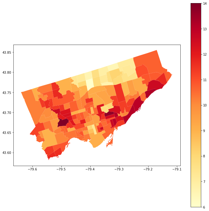
Hmm - Looks like there are some spatial patterns!

We can also look at non-spatial figures to explore our data. Doing this helps us understand the ‘shape’ of our data in different ways.

Let’s create a histogram of the same data in the following cell:

# Just like what we do in pandas
nbrhd_simple['asthma_pct'].hist(bins=8)

plt.xlabel('Asthma Percent')
plt.ylabel('Number of neighbourhoods')
plt.title('Distribution of percent of residents with asthma in Toronto, ON')
plt.show()

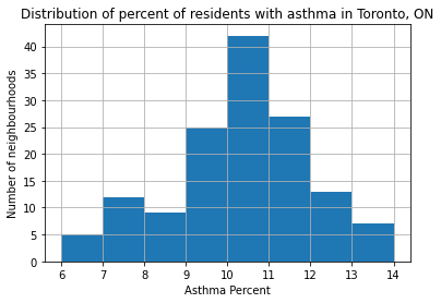
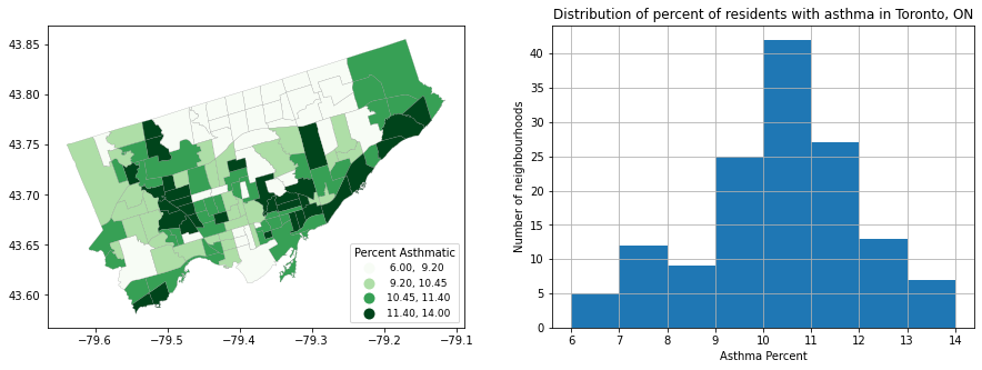
Interesting!

This looks like a “normal” distribution:

• Many neighbourhoods with values in the middle range, but some at the extremes (both low and high).

But when we look at the map, we notice that neighbourhoods with high values tend to be near other neighbourhoods with high values, and low value neighbourhoods near others with low values.

Maybe there is some spatial mechanism causing this!

To dig into this more, let’s classify the data using quartiles…

To do this we add a scheme parameter to the plot function and use quantiles. the k value tells the plot function how many quantiles you want. We want four quantiles (0-25%, 25%-50%, 50%-75%, 75%-100%).

More information about plot function

We do this for a few reasons:

• (1) It makes it easier to see groups with similar values that are close to eachother and

• (2) it makes the legend easier to interpret.

Note that we also have added an edgecolor parameter which tells the map what color to outline neighbourhoods with.

fig, axes = plt.subplots(1,1, figsize =  (10,10))
nbrhd_simple.plot(column='asthma_pct', scheme='quantiles', 
                  k=4, cmap='YlOrRd', edgecolor='black', 
                  ax = axes, legend=True)

<AxesSubplot:>

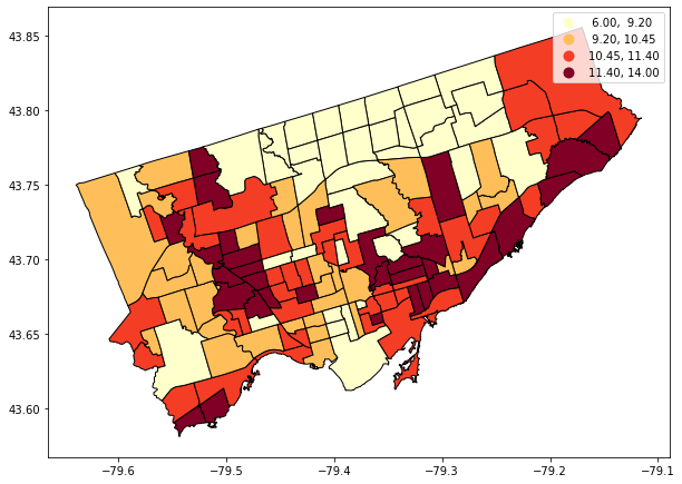
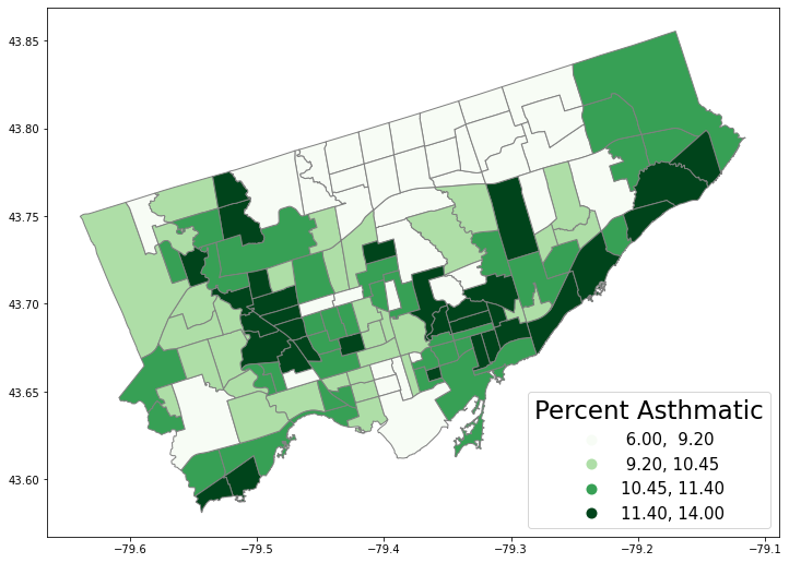
This map looks a lot better, I think! But the legend is overlapping the map. We should move it.

The legend options are kind of complicated, but you can find more about stuff here: https://matplotlib.org/3.5.1/api/_as_gen/matplotlib.pyplot.legend.html

I’m going to show you a few things you can do, like move the legend, adjust font size, and add a title:

fig, axes = plt.subplots(1,1, figsize =  (12,12))

nbrhd_simple.plot(column='asthma_pct', scheme='quantiles', 
                  k=4, cmap='Greens', edgecolor='grey', 
                  ax = axes, legend=True, 
                  legend_kwds={'loc': 4, 'title': 'Percent Asthmatic',
                               'title_fontsize': 23,'fontsize': 15}) #'loc'=4 means lower right

<AxesSubplot:>

Can we show descriptive stats charts next to a map?

Yes!

#First create a figure sheet with 2 axes cells (and resize the figure)
fig, axes = plt.subplots(1,2, figsize = (15,5))

#let's put the map in the first axes cell:
nbrhd_simple.plot(column='asthma_pct', scheme='quantiles', 
                  k=4, cmap='Greens', edgecolor='grey', linewidth = 0.2, #notice I added linewidth to narrow the borders
                  ax = axes[0], legend=True, 
                  legend_kwds={'loc': 4, 'title': 'Percent Asthmatic', 
                               'title_fontsize': 10,'fontsize': 9})

#we can put the histogram we made earlier in the second axes cell:
nbrhd_simple['asthma_pct'].hist(bins=8, ax = axes[1])
plt.xlabel('Asthma Percent')
plt.ylabel('Number of neighbourhoods')
plt.title('Distribution of percent of residents with asthma in Toronto, ON')

Text(0.5, 1.0, 'Distribution of percent of residents with asthma in Toronto, ON')

First steps into “spatial analysis”…

OK great! That chart is interesting and gets us thinking. But one of the powers of spatial analysis is relating environments to spatial phenomena.

What might be related to these areas with higher asthma?

Let’s make a map with multiple layers of info…

To do this, we need a second spatial data file. We know there is research that relates asthma to being near railroads. Let’s see if being near a railway in Toronto is associated to patterns of asthma.

#first we need to bring in the spatial data on railroads in the Toronto area

railways = gpd.GeoDataFrame.from_file("toronto_rails.geojson")
railways.plot()

<AxesSubplot:>

Coordinate systems and projections

When working with spatial data, you may need to think about coordinate systems and geographic projections.

Because we are taking data that exist on a sphere and laying them out flat on a plane, all spatial data is projected.

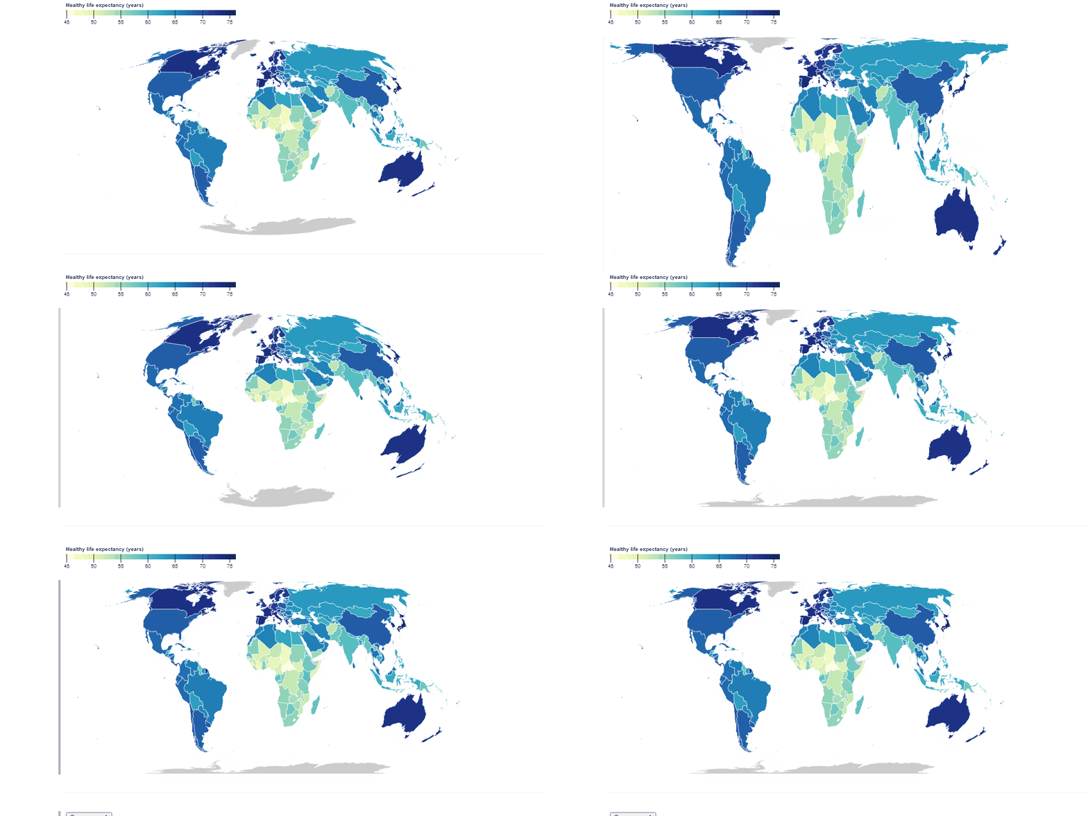
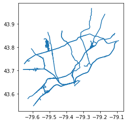
If you have two layers of spatial data it is always good to check that they are in the same projection, or else you will get errors or bad results.

If the files are not in the same projection, it’s pretty simple to convert one of the files to the same projection as the other file:

# double check coordinate systems - we always want to work in the same projection

print("The original projection of railways is: ", railways.crs)
print("The original projection of nbrhd_simple is: ", nbrhd_simple.crs)

# reproject railways so it's the same as our neighbourhood layer
railways = railways.to_crs(nbrhd_simple.crs) #we can just borrow the "crs" (coordinate reference system) from the other spatial file
print("The NEW projection of railways is: ", railways.crs)
print("And nbrhd_simple is still: ", nbrhd_simple.crs)
railways.plot()

The original projection of railways is:  EPSG:4269
The original projection of nbrhd_simple is:  EPSG:4326
The NEW projection of railways is:  EPSG:4326
And nbrhd_simple is still:  EPSG:4326

<AxesSubplot:>

nbrhd_simple.head()

	name_x	nbrhd_spat_id	geometry	Neighbid	name_y	asthma_pct
0	Casa Loma (96)	096	POLYGON ((-79.41469 43.67391, -79.41485 43.674...	96	Casa Loma	10.1
1	Annex (95)	095	POLYGON ((-79.39414 43.66872, -79.39588 43.668...	95	Annex	9.5
2	Caledonia-Fairbank (109)	109	POLYGON ((-79.46021 43.68156, -79.46044 43.681...	109	Caledonia-Fairbank	11.3
3	Woodbine Corridor (64)	064	POLYGON ((-79.31485 43.66674, -79.31660 43.666...	64	Woodbine Corridor	13.0
4	Lawrence Park South (103)	103	POLYGON ((-79.41096 43.70408, -79.41165 43.703...	103	Lawrence Park South	10.7

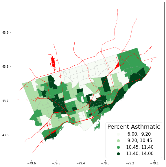
Now that our two geodataframe spatial layers are in the same projection, we can plot them together

We want to create 1 map and tell geopandas to put the two spatial layers in the same axes cell:

fig, axes = plt.subplots(1,1, figsize = (15,10))



nbrhd_simple.plot(column='asthma_pct', scheme='quantiles', 
                  k=4, cmap='Greens', edgecolor='grey',
                  linewidth = .2, ax = axes, legend=True, 
                  legend_kwds={'loc': 4, 'title': 'Percent Asthmatic', 
                               'title_fontsize': 20,'fontsize': 15})

railways.plot(edgecolor="red", linewidth = .5, ax = axes) #notice i'm putting this in the same axes cell

<AxesSubplot:>

railways.columns

Index(['OBJECTID', 'OGF_ID', 'TRACKNID', 'TRACKSEGID', 'TRACKNAME',
       'TRACKCLASS', 'REGULATOR', 'TRANSPTYPE', 'USETYPE', 'GAUGE',
       'NUMTRACKS', 'ELECTRIC', 'STATUS', 'SPEEDFREIT', 'SPEEDPASSE',
       'UNITOFSPEE', 'SOURCEID', 'OPERATOENA', 'OPERATOFNA', 'OPERATORMK',
       'OPSUBSTART', 'OPSUBEND', 'OPSUBUDIS', 'OWNERENA', 'OWNERFNA',
       'TRKUSR1ENA', 'TRKUSR1FNA', 'TRKUSR1RMK', 'TRKUSR2ENA', 'TRKUSR2FNA',
       'TRKUSR2RMK', 'TRKUSR3ENA', 'TRKUSR3FNA', 'TRKUSR3RMK', 'TRKUSR4ENA',
       'TRKUSR4FNA', 'TRKUSR4RMK', 'SUBDI1NID', 'SUBDI1NAME', 'SUBD1START',
       'SUBD1END', 'SUB1UNITDI', 'SUBDI2NID', 'SUBDI2NAME', 'SUBD2START',
       'SUBD2END', 'SUB2UNITDI', 'ADMINAREA', 'SPECVERS', 'SECURCLASS',
       'GEOCREDATE', 'GEOREVDATE', 'GEOACQTECH', 'GEOACCURA', 'GEOPROVIDE',
       'ATTCREDATE', 'ATTREVDATE', 'ATTACQTECH', 'ATTPROVIDE', 'EFFECTIVE_',
       'SHAPE_Leng', 'SHAPE_1_Le', 'geometry'],
      dtype='object')

Hmm - could there be something there?

Maybe!

But what are the things that might be happening here?

Let’s do a “spatial join”

What is a spatial join?

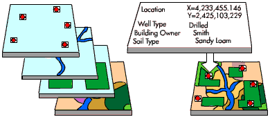
Basically, we are relating information from two tables that share a spatial relationship.

So information from layer a’s table will be joined with information from layer b’s table where the two intersect/touch/are within/etc.

We will use “intersect” here, but you can refer to the geopandas documentation to learn more:

https://geopandas.org/en/stable/gallery/spatial_joins.html

join_left_df = nbrhd_simple.sjoin(railways, how="left", predicate = "intersects")
join_left_df

	name_x	nbrhd_spat_id	geometry	Neighbid	name_y	asthma_pct	index_right	OBJECTID	OGF_ID	TRACKNID	...	GEOACQTECH	GEOACCURA	GEOPROVIDE	ATTCREDATE	ATTREVDATE	ATTACQTECH	ATTPROVIDE	EFFECTIVE_	SHAPE_Leng	SHAPE_1_Le
0	Casa Loma (96)	096	POLYGON ((-79.41469 43.67391, -79.41485 43.674...	96	Casa Loma	10.1	1280.0	1720.0	10131.0	2579cdd5ccaf447e93bec017362a451a	...	Vector Data	10.0	Provincial/Territorial	201306	None	Vector Data	Federal	2013-07-30	0.0	0.026163
0	Casa Loma (96)	096	POLYGON ((-79.41469 43.67391, -79.41485 43.674...	96	Casa Loma	10.1	3222.0	8267.0	16018.0	ced49be659214db99e606ea1f3153f03	...	Vector Data	10.0	Provincial/Territorial	201306	None	Vector Data	Federal	2013-07-30	0.0	0.043467
0	Casa Loma (96)	096	POLYGON ((-79.41469 43.67391, -79.41485 43.674...	96	Casa Loma	10.1	888.0	9370.0	17250.0	05f860e758f746be971872822cb137c8	...	Vector Data	10.0	Provincial/Territorial	201306	None	Vector Data	Federal	2013-07-30	0.0	0.060344
0	Casa Loma (96)	096	POLYGON ((-79.41469 43.67391, -79.41485 43.674...	96	Casa Loma	10.1	1844.0	10459.0	3086.0	1fd8c25a828f46829c173713f49c63d3	...	Vector Data	10.0	Provincial/Territorial	201306	None	Vector Data	Federal	2013-07-30	0.0	0.008783
1	Annex (95)	095	POLYGON ((-79.39414 43.66872, -79.39588 43.668...	95	Annex	9.5	1280.0	1720.0	10131.0	2579cdd5ccaf447e93bec017362a451a	...	Vector Data	10.0	Provincial/Territorial	201306	None	Vector Data	Federal	2013-07-30	0.0	0.026163
...	...	...	...	...	...	...	...	...	...	...	...	...	...	...	...	...	...	...	...	...	...
137	Humbermede (22)	022	POLYGON ((-79.52628 43.73640, -79.52649 43.736...	22	Humbermede	10.8	1239.0	9798.0	2436.0	816b3f97bace44149b88174dc78a7e55	...	Orthoimage	10.0	Federal	201306	None	Vector Data	Federal	2013-07-30	0.0	0.002236
137	Humbermede (22)	022	POLYGON ((-79.52628 43.73640, -79.52649 43.736...	22	Humbermede	10.8	2305.0	15763.0	8280.0	9da306e9415d4e7fa5b006a39dc550c1	...	Orthoimage	10.0	Federal	201306	None	Vector Data	Federal	2013-07-30	0.0	0.002528
137	Humbermede (22)	022	POLYGON ((-79.52628 43.73640, -79.52649 43.736...	22	Humbermede	10.8	717.0	5591.0	13590.0	632d434dd2b24ef5aaf8544d87f467f5	...	Orthoimage	10.0	Federal	201306	None	Vector Data	Federal	2013-07-30	0.0	0.012516
138	Willowdale West (37)	037	POLYGON ((-79.44043 43.76340, -79.44052 43.763...	37	Willowdale West	8.0	NaN	NaN	NaN	NaN	...	NaN	NaN	NaN	NaN	NaN	NaN	NaN	NaN	NaN	NaN
139	Willowdale East (51)	051	POLYGON ((-79.41225 43.76669, -79.41232 43.766...	51	Willowdale East	6.0	NaN	NaN	NaN	NaN	...	NaN	NaN	NaN	NaN	NaN	NaN	NaN	NaN	NaN	NaN

2528 rows × 69 columns

join_left_df.loc[join_left_df['TRACKNID'].isnull()]

	name_x	nbrhd_spat_id	geometry	Neighbid	name_y	asthma_pct	index_right	OBJECTID	OGF_ID	TRACKNID	...	GEOACQTECH	GEOACCURA	GEOPROVIDE	ATTCREDATE	ATTREVDATE	ATTACQTECH	ATTPROVIDE	EFFECTIVE_	SHAPE_Leng	SHAPE_1_Le
4	Lawrence Park South (103)	103	POLYGON ((-79.41096 43.70408, -79.41165 43.703...	103	Lawrence Park South	10.7	NaN	NaN	NaN	NaN	...	NaN	NaN	NaN	NaN	NaN	NaN	NaN	NaN	NaN	NaN
6	Henry Farm (53)	053	POLYGON ((-79.35966 43.76649, -79.35966 43.766...	53	Henry Farm	6.7	NaN	NaN	NaN	NaN	...	NaN	NaN	NaN	NaN	NaN	NaN	NaN	NaN	NaN	NaN
10	Pleasant View (46)	046	POLYGON ((-79.34346 43.79517, -79.34359 43.795...	46	Pleasant View	7.7	NaN	NaN	NaN	NaN	...	NaN	NaN	NaN	NaN	NaN	NaN	NaN	NaN	NaN	NaN
11	Steeles (116)	116	POLYGON ((-79.34132 43.81565, -79.33988 43.816...	116	Steeles	6.5	NaN	NaN	NaN	NaN	...	NaN	NaN	NaN	NaN	NaN	NaN	NaN	NaN	NaN	NaN
13	Brookhaven-Amesbury (30)	030	POLYGON ((-79.50296 43.69574, -79.50415 43.696...	30	Brookhaven-Amesbury	12.2	NaN	NaN	NaN	NaN	...	NaN	NaN	NaN	NaN	NaN	NaN	NaN	NaN	NaN	NaN
16	Yonge-Eglinton (100)	100	POLYGON ((-79.41096 43.70408, -79.40962 43.704...	100	Yonge-Eglinton	10.8	NaN	NaN	NaN	NaN	...	NaN	NaN	NaN	NaN	NaN	NaN	NaN	NaN	NaN	NaN
18	Englemount-Lawrence (32)	032	POLYGON ((-79.43854 43.70586, -79.43855 43.705...	32	Englemount-Lawrence	10.1	NaN	NaN	NaN	NaN	...	NaN	NaN	NaN	NaN	NaN	NaN	NaN	NaN	NaN	NaN
19	Bridle Path-Sunnybrook-York Mills (41)	041	POLYGON ((-79.39008 43.72768, -79.39016 43.728...	41	Bridle Path-Sunnybrook-York Mills	9.2	NaN	NaN	NaN	NaN	...	NaN	NaN	NaN	NaN	NaN	NaN	NaN	NaN	NaN	NaN
21	Danforth East York (59)	059	POLYGON ((-79.34627 43.68272, -79.34645 43.683...	59	Danforth Village-East York	12.5	NaN	NaN	NaN	NaN	...	NaN	NaN	NaN	NaN	NaN	NaN	NaN	NaN	NaN	NaN
22	Elms-Old Rexdale (5)	005	POLYGON ((-79.55512 43.71510, -79.55569 43.716...	5	Elms-Old Rexdale	11.6	NaN	NaN	NaN	NaN	...	NaN	NaN	NaN	NaN	NaN	NaN	NaN	NaN	NaN	NaN
24	North St.James Town (74)	074	POLYGON ((-79.38057 43.67161, -79.37947 43.671...	74	North St. James Town	8.9	NaN	NaN	NaN	NaN	...	NaN	NaN	NaN	NaN	NaN	NaN	NaN	NaN	NaN	NaN
25	Highland Creek (134)	134	POLYGON ((-79.17527 43.78021, -79.17535 43.780...	134	Highland Creek	10.8	NaN	NaN	NaN	NaN	...	NaN	NaN	NaN	NaN	NaN	NaN	NaN	NaN	NaN	NaN
27	Don Valley Village (47)	047	POLYGON ((-79.36414 43.77164, -79.36412 43.771...	47	Don Valley Village	7.2	NaN	NaN	NaN	NaN	...	NaN	NaN	NaN	NaN	NaN	NaN	NaN	NaN	NaN	NaN
28	Mount Pleasant West (104)	104	POLYGON ((-79.39611 43.69566, -79.39620 43.696...	104	Mount Pleasant West	8.6	NaN	NaN	NaN	NaN	...	NaN	NaN	NaN	NaN	NaN	NaN	NaN	NaN	NaN	NaN
29	Westminster-Branson (35)	035	POLYGON ((-79.44043 43.76340, -79.44004 43.761...	35	Westminster-Branson	7.3	NaN	NaN	NaN	NaN	...	NaN	NaN	NaN	NaN	NaN	NaN	NaN	NaN	NaN	NaN
41	Bay Street Corridor (76)	076	POLYGON ((-79.38752 43.65067, -79.38663 43.650...	76	Bay Street Corridor	7.3	NaN	NaN	NaN	NaN	...	NaN	NaN	NaN	NaN	NaN	NaN	NaN	NaN	NaN	NaN
42	Bathurst Manor (34)	034	POLYGON ((-79.43998 43.76156, -79.43967 43.761...	34	Bathurst Manor	9.2	NaN	NaN	NaN	NaN	...	NaN	NaN	NaN	NaN	NaN	NaN	NaN	NaN	NaN	NaN
44	L'Amoreaux (117)	117	POLYGON ((-79.28857 43.79607, -79.28921 43.795...	117	L'Amoreaux	8.1	NaN	NaN	NaN	NaN	...	NaN	NaN	NaN	NaN	NaN	NaN	NaN	NaN	NaN	NaN
45	Trinity-Bellwoods (81)	081	POLYGON ((-79.42241 43.64349, -79.42255 43.643...	81	Trinity-Bellwoods	9.5	NaN	NaN	NaN	NaN	...	NaN	NaN	NaN	NaN	NaN	NaN	NaN	NaN	NaN	NaN
47	Glenfield-Jane Heights (25)	025	POLYGON ((-79.52628 43.73640, -79.52721 43.740...	25	Glenfield-Jane Heights	11.7	NaN	NaN	NaN	NaN	...	NaN	NaN	NaN	NaN	NaN	NaN	NaN	NaN	NaN	NaN
49	Eringate-Centennial-West Deane (11)	011	POLYGON ((-79.56730 43.65425, -79.56755 43.654...	11	Eringate-Centennial-West Deane	11.2	NaN	NaN	NaN	NaN	...	NaN	NaN	NaN	NaN	NaN	NaN	NaN	NaN	NaN	NaN
54	Taylor-Massey (61)	061	POLYGON ((-79.28776 43.68978, -79.29269 43.688...	61	Crescent Town	9.9	NaN	NaN	NaN	NaN	...	NaN	NaN	NaN	NaN	NaN	NaN	NaN	NaN	NaN	NaN
55	Humewood-Cedarvale (106)	106	POLYGON ((-79.41849 43.68363, -79.41913 43.683...	106	Humewood-Cedarvale	10.8	NaN	NaN	NaN	NaN	...	NaN	NaN	NaN	NaN	NaN	NaN	NaN	NaN	NaN	NaN
60	Rustic (28)	028	POLYGON ((-79.50384 43.70288, -79.50425 43.704...	28	Rustic	11.5	NaN	NaN	NaN	NaN	...	NaN	NaN	NaN	NaN	NaN	NaN	NaN	NaN	NaN	NaN
62	Forest Hill North (102)	102	POLYGON ((-79.42556 43.70099, -79.42669 43.700...	102	Forest Hill North	8.9	NaN	NaN	NaN	NaN	...	NaN	NaN	NaN	NaN	NaN	NaN	NaN	NaN	NaN	NaN
63	Hillcrest Village (48)	048	POLYGON ((-79.34346 43.79517, -79.34351 43.795...	48	Hillcrest Village	6.9	NaN	NaN	NaN	NaN	...	NaN	NaN	NaN	NaN	NaN	NaN	NaN	NaN	NaN	NaN
64	Humber Heights-Westmount (8)	008	POLYGON ((-79.51329 43.69338, -79.51330 43.692...	8	Humber Heights-Westmount	9.8	NaN	NaN	NaN	NaN	...	NaN	NaN	NaN	NaN	NaN	NaN	NaN	NaN	NaN	NaN
65	Danforth (66)	066	POLYGON ((-79.32364 43.68337, -79.32477 43.683...	66	Danforth Village-Toronto	11.0	NaN	NaN	NaN	NaN	...	NaN	NaN	NaN	NaN	NaN	NaN	NaN	NaN	NaN	NaN
66	Newtonbrook West (36)	036	POLYGON ((-79.44576 43.79241, -79.44335 43.792...	36	Newtonbrook West	7.2	NaN	NaN	NaN	NaN	...	NaN	NaN	NaN	NaN	NaN	NaN	NaN	NaN	NaN	NaN
67	Black Creek (24)	024	POLYGON ((-79.53488 43.77269, -79.53441 43.772...	24	Black Creek	11.5	NaN	NaN	NaN	NaN	...	NaN	NaN	NaN	NaN	NaN	NaN	NaN	NaN	NaN	NaN
68	University (79)	079	POLYGON ((-79.40772 43.65648, -79.40847 43.658...	79	University	8.1	NaN	NaN	NaN	NaN	...	NaN	NaN	NaN	NaN	NaN	NaN	NaN	NaN	NaN	NaN
70	Kensington-Chinatown (78)	078	POLYGON ((-79.40401 43.64719, -79.40419 43.647...	78	Kensington-Chinatown	8.6	NaN	NaN	NaN	NaN	...	NaN	NaN	NaN	NaN	NaN	NaN	NaN	NaN	NaN	NaN
71	Old East York (58)	058	POLYGON ((-79.35056 43.69941, -79.35041 43.699...	58	Old East York	13.7	NaN	NaN	NaN	NaN	...	NaN	NaN	NaN	NaN	NaN	NaN	NaN	NaN	NaN	NaN
74	Palmerston-Little Italy (80)	080	POLYGON ((-79.42640 43.65360, -79.42744 43.656...	80	Palmerston-Little Italy	10.4	NaN	NaN	NaN	NaN	...	NaN	NaN	NaN	NaN	NaN	NaN	NaN	NaN	NaN	NaN
78	Bedford Park-Nortown (39)	039	POLYGON ((-79.40493 43.73601, -79.40503 43.735...	39	Bedford Park-Nortown	10.2	NaN	NaN	NaN	NaN	...	NaN	NaN	NaN	NaN	NaN	NaN	NaN	NaN	NaN	NaN
83	Willowridge-Martingrove-Richview (7)	007	POLYGON ((-79.52661 43.68233, -79.52705 43.682...	7	Willowridge-Martingrove-Richview	9.9	NaN	NaN	NaN	NaN	...	NaN	NaN	NaN	NaN	NaN	NaN	NaN	NaN	NaN	NaN
84	Woodbine-Lumsden (60)	060	POLYGON ((-79.31743 43.69644, -79.31775 43.697...	60	Woodbine-Lumsden	13.1	NaN	NaN	NaN	NaN	...	NaN	NaN	NaN	NaN	NaN	NaN	NaN	NaN	NaN	NaN
91	Morningside (135)	135	POLYGON ((-79.22552 43.78925, -79.22549 43.789...	135	Morningside	10.9	NaN	NaN	NaN	NaN	...	NaN	NaN	NaN	NaN	NaN	NaN	NaN	NaN	NaN	NaN
93	Lawrence Park North (105)	105	POLYGON ((-79.39008 43.72768, -79.39199 43.727...	105	Lawrence Park North	11.5	NaN	NaN	NaN	NaN	...	NaN	NaN	NaN	NaN	NaN	NaN	NaN	NaN	NaN	NaN
94	Clanton Park (33)	033	POLYGON ((-79.43371 43.73615, -79.43626 43.734...	33	Clanton Park	9.8	NaN	NaN	NaN	NaN	...	NaN	NaN	NaN	NaN	NaN	NaN	NaN	NaN	NaN	NaN
96	Markland Wood (12)	012	POLYGON ((-79.55959 43.63624, -79.55957 43.636...	12	Markland Wood	10.6	NaN	NaN	NaN	NaN	...	NaN	NaN	NaN	NaN	NaN	NaN	NaN	NaN	NaN	NaN
97	Maple Leaf (29)	029	POLYGON ((-79.49249 43.72010, -79.49185 43.720...	29	Maple Leaf	10.2	NaN	NaN	NaN	NaN	...	NaN	NaN	NaN	NaN	NaN	NaN	NaN	NaN	NaN	NaN
101	Etobicoke West Mall (13)	013	POLYGON ((-79.55959 43.63624, -79.55980 43.636...	13	Etobicoke West Mall	9.8	NaN	NaN	NaN	NaN	...	NaN	NaN	NaN	NaN	NaN	NaN	NaN	NaN	NaN	NaN
107	Church-Yonge Corridor (75)	075	POLYGON ((-79.37672 43.66242, -79.37658 43.662...	75	Church-Yonge Corridor	9.8	NaN	NaN	NaN	NaN	...	NaN	NaN	NaN	NaN	NaN	NaN	NaN	NaN	NaN	NaN
112	Newtonbrook East (50)	050	POLYGON ((-79.42008 43.79800, -79.41973 43.798...	50	Newtonbrook East	6.6	NaN	NaN	NaN	NaN	...	NaN	NaN	NaN	NaN	NaN	NaN	NaN	NaN	NaN	NaN
119	Oakwood Village (107)	107	POLYGON ((-79.45028 43.69569, -79.44934 43.695...	107	Oakwood-Vaughan	10.7	NaN	NaN	NaN	NaN	...	NaN	NaN	NaN	NaN	NaN	NaN	NaN	NaN	NaN	NaN
121	Mount Pleasant East (99)	099	POLYGON ((-79.37749 43.71309, -79.37739 43.712...	99	Mount Pleasant East	10.5	NaN	NaN	NaN	NaN	...	NaN	NaN	NaN	NaN	NaN	NaN	NaN	NaN	NaN	NaN
122	Rexdale-Kipling (4)	004	POLYGON ((-79.55512 43.71510, -79.55504 43.714...	4	Rexdale-Kipling	11.4	NaN	NaN	NaN	NaN	...	NaN	NaN	NaN	NaN	NaN	NaN	NaN	NaN	NaN	NaN
124	Thistletown-Beaumond Heights (3)	003	POLYGON ((-79.57751 43.73384, -79.57806 43.734...	3	Thistletown-Beaumond Heights	10.0	NaN	NaN	NaN	NaN	...	NaN	NaN	NaN	NaN	NaN	NaN	NaN	NaN	NaN	NaN
125	The Beaches (63)	063	POLYGON ((-79.31485 43.66674, -79.31356 43.667...	63	The Beaches	11.4	NaN	NaN	NaN	NaN	...	NaN	NaN	NaN	NaN	NaN	NaN	NaN	NaN	NaN	NaN
128	Forest Hill South (101)	101	POLYGON ((-79.42556 43.70099, -79.42314 43.701...	101	Forest Hill South	10.3	NaN	NaN	NaN	NaN	...	NaN	NaN	NaN	NaN	NaN	NaN	NaN	NaN	NaN	NaN
129	Princess-Rosethorn (10)	010	POLYGON ((-79.52679 43.65093, -79.52688 43.650...	10	Princess-Rosethorn	10.4	NaN	NaN	NaN	NaN	...	NaN	NaN	NaN	NaN	NaN	NaN	NaN	NaN	NaN	NaN
130	Lansing-Westgate (38)	038	POLYGON ((-79.43998 43.76156, -79.44004 43.761...	38	Lansing-Westgate	9.0	NaN	NaN	NaN	NaN	...	NaN	NaN	NaN	NaN	NaN	NaN	NaN	NaN	NaN	NaN
138	Willowdale West (37)	037	POLYGON ((-79.44043 43.76340, -79.44052 43.763...	37	Willowdale West	8.0	NaN	NaN	NaN	NaN	...	NaN	NaN	NaN	NaN	NaN	NaN	NaN	NaN	NaN	NaN
139	Willowdale East (51)	051	POLYGON ((-79.41225 43.76669, -79.41232 43.766...	51	Willowdale East	6.0	NaN	NaN	NaN	NaN	...	NaN	NaN	NaN	NaN	NaN	NaN	NaN	NaN	NaN	NaN

55 rows × 69 columns

Woah!

Now we have 2528 rows… that’s way more rows than neighbourhoods. What happened?

Spatial join creates a new row for every instance of ‘intersection’. So if railway 1 and railway 2 both go through neighbourhood a, then there will be two rows with neighbourhood a with one row joined with railway a data and the other joined with railway b data.

Also, notice that neighbourhoods that didn’t have any railway go through them were appended with NaNs. This is saying there is no data about railways for these neighbourhoods because there were none there.

Because we just want to know what neighbourhoods have ANY railway go through them, we can take the joined results and remove duplicate rows of each neighbourhood.

no_duplicates_gdf = join_left_df.copy()
no_duplicates_gdf = no_duplicates_gdf.drop_duplicates('Neighbid')
no_duplicates_gdf.shape

(140, 69)

Let’s check this new, no duplicate geodataframe to see if looks right.

We can plot the map using “index_right” which is the index from the railway layer. The values are meaningless, but it shows us where there ARE values and where there are not.

no_duplicates_gdf.plot(column = "index_right")

<AxesSubplot:>

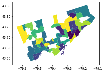
This looks good, based on visual inspection

But we need a column that tells us there IS or there IS NOT a railway in each neighbourhood. We can go back to some of the skills we learned earlier in the course to do this.

We will first create two series of TRUE and FALSE values to show where a value exists in the “index_right” column.

The series rail_present will be true if there is a value in the column - implying a railway goes through the neighbourhood, and false otherwise.

The series rail_not_present will be true if there is a NaN value in the row where the railway info is, and false otherwise.

rail_present = no_duplicates_gdf["index_right"] >= 0
rail_present.value_counts()

True     85
False    55
Name: index_right, dtype: int64

rail_not_present = no_duplicates_gdf["index_right"].isnull()
rail_not_present.value_counts()

False    85
True     55
Name: index_right, dtype: int64

Let’s clean things up a little and create the final geodataframe we want to work with

We can clean things up and then create a map and a descriptive statistics plot to show our findings.

#create list of columns relevant to our analysis
columns_to_keep = ["name_x","Neighbid","name_y","asthma_pct","index_right","geometry"]

#create our final analysis geodataframe and create a column 'rail_present' that is true 
#if railways are in the neighbourhood and false if not:
final_toronto_analysis = no_duplicates_gdf[columns_to_keep].copy()
final_toronto_analysis.loc[rail_present, 'rail_present'] = True
final_toronto_analysis.loc[rail_not_present, 'rail_present'] = False
final_toronto_analysis.head()

	name_x	Neighbid	name_y	asthma_pct	index_right	geometry	rail_present
0	Casa Loma (96)	96	Casa Loma	10.1	1280.0	POLYGON ((-79.41469 43.67391, -79.41485 43.674...	True
1	Annex (95)	95	Annex	9.5	1280.0	POLYGON ((-79.39414 43.66872, -79.39588 43.668...	True
2	Caledonia-Fairbank (109)	109	Caledonia-Fairbank	11.3	1305.0	POLYGON ((-79.46021 43.68156, -79.46044 43.681...	True
3	Woodbine Corridor (64)	64	Woodbine Corridor	13.0	1940.0	POLYGON ((-79.31485 43.66674, -79.31660 43.666...	True
4	Lawrence Park South (103)	103	Lawrence Park South	10.7	NaN	POLYGON ((-79.41096 43.70408, -79.41165 43.703...	False

fig, axes = plt.subplots(1,2, figsize = (15,7))

final_toronto_analysis.boxplot(column="asthma_pct", 
                               by = "rail_present", 
                               ax = axes[0])

final_toronto_analysis.plot(column='asthma_pct', scheme='quantiles', 
                  k=2, cmap='Greens', edgecolor='grey', linewidth = 0.2, 
                  ax = axes[1], legend=True, 
                  legend_kwds={'loc': 4, 'title': 'Percent Asthmatic', 
                               'title_fontsize': 14,'fontsize': 11})
railways.plot(ax=axes[1], edgecolor='red',linewidth=0.5)

axes[0].set_title("")
axes[0].set_ylabel("Asthma Percent", fontsize = 15)
axes[0].set_xlabel("Rail Present?", fontsize = 15)

fig.suptitle("Percent of Population with Asthma for Neighbourhoods with Railways", 
             fontsize = 20, fontweight = "bold")

Text(0.5, 0.98, 'Percent of Population with Asthma for Neighbourhoods with Railways')

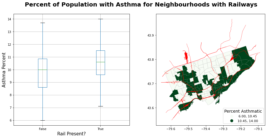
It seems that the presence of railway in neighborhood is related to higher asthma rate!

But is it a significant relationship?

Remember the comparison between two groups before!

Let’s do a hypothesis testing using shuffling method.

• Null hypothesis: There is no differences of asthma rates between neighborhoods with railways and without railways.

• Alternative hypothesis: Neighborhoods with railways have higher asthma rates than the neighborhoods without railways.

Let’s do a exercise.

# Simulation
simulated_diffs = []

for _ in range(5000):
    simulated = final_toronto_analysis['rail_present'].sample(frac=1, replace = False).reset_index(drop = True)
    mean_railway = final_toronto_analysis.loc[simulated == True, 'asthma_pct'].mean()
    mean_norailway = final_toronto_analysis.loc[simulated == False, 'asthma_pct'].mean()
    sim_diff = mean_railway - mean_norailway
    simulated_diffs.append(sim_diff)

# Calculate observed difference
obs_mean_railway = final_toronto_analysis.loc[final_toronto_analysis['rail_present'] == True, 'asthma_pct'].mean()
obs_mean_norailway = final_toronto_analysis.loc[final_toronto_analysis['rail_present'] == False, 'asthma_pct'].mean()

obs_diff = obs_mean_railway - obs_mean_norailway

# Calculate p-value
simulated_diffs_df = pd.DataFrame({'sim_diffs' : simulated_diffs})

numgreater = (simulated_diffs_df['sim_diffs'] >= obs_diff).sum()
print('The number of simulated differences greater than the observed difference is:', numgreater)

numsmaller = (simulated_diffs_df['sim_diffs'] < -1 * obs_diff).sum()
print('The number of simulated differences smaller than the observed difference is:', numsmaller)

pvalue = (numgreater + numsmaller)/ 5000

print('The p-value is:', pvalue)

The number of simulated differences greater than the observed difference is: 11
The number of simulated differences smaller than the observed difference is: 13
The p-value is: 0.0048

Great! We can say the asthma rates in neighborhoods with railways are significantly higher than the rates in neighborhoods without railways.

But is this a causal relationship?